3D-shepp-logan-phantom

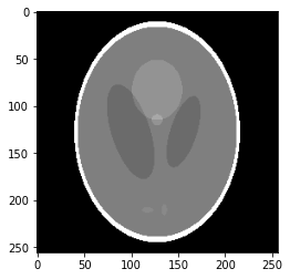
The Shepp-Logan phantom consists of several elliptical sections that can simulate different densities and structures, such as bones, soft tissues or voids inside the human body. Each ellipse in the phantom has specific parameters, such as position, orientation, size and absorption coefficient, which allows it to faithfully mimic the way X-rays are absorbed by different tissue types.

Any parallel projection in 3D space can be regarded as a projection made in the (x, y) plane by a beam of radiation parallel to the x-axis, after all the rays of the beam have been subjected to two transformations combined. The first of these transformations is rotation in the (x, y) plane by an angle a1 p about the z-axis. This means that the coordinate system (x, y, z) can be replaced by the rotated system (s, u, z),

Ellipse	x0	y0	z0	a	b	c	Theta	Gray level
I	0.000	0.000	0.000	0.6900	0.9200	0.9000	0.0	2.00
II	0.000	0.000	0.000	0.6624	0.8740	0.8800	0.0	-0.98
III	-0.220	0.000	-0.250	0.4100	0.1600	0.2100	108.0	-0.02
IV	0.220	0.000	-0.250	0.3100	0.1100	0.2200	72.0	-0.02
V	0.000	0.350	-0.250	0.2100	0.2500	0.5000	0.0	0.02
VI	0.000	0.100	-0.250	0.0460	0.0460	0.0460	0.0	0.02
VII	-0.080	-0.650	-0.250	0.0460	0.0230	0.0200	0.0	0.01
VIII	0.060	-0.650	-0.250	0.0230	0.0460	0.0200	90.0	0.01
IX	0.060	-0.105	0.625	0.0400	0.0560	0.1000	90.0	0.02
X	0.000	0.100	0.625	0.0560	0.0400	0.1000	0.0	-0.02

The 3D Shepp-Logan model can be described by mathematical equations that define ellipses. The parameters of each ellipse, such as the position of the center, the axes, the angle of inclination and the absorption coefficient, are precisely defined.

$$ s = x \cos \alpha^p_1 $$

and

$$ u = - \sin \alpha^p_1 + y \cos \alpha^p_1 $$

The second transformation is rotation of the (s, u, z) system by an angle (a_2 p) about the s axis. If we introduce a new, rotated coordinate system ((s, u', t)), the coordinates of any point in this space can be calculated using the following relationships:

$$t = z \cos a_p^2 + \left( -x \sin a_p^1 + y \cos a_p^1 \right) \sin a_p^2 \quad $$

and

$$ u' = -z \sin a_p^2 + \left( -x \sin a_p^1 + y \cos a_p^1 \right) \cos a_p^2 \quad $$

See more in book[1]

References

[1] Robert Cierniak (2011), X-Ray Computed Tomography in Biomedical Engineering, Springer, ISBN: 9780857290267