| layout | title | description |
|---|---|---|
default |
Base Results |
Results by Parcellation Type |
To model the base results with respect to type of parcellation we use an OLS regression, with
the formula log10(Mean_Rank) ~ log10(Size) + C(Parcellation_Type), so notably first treating choice of parcellation as a fixed effect.
We first though estimate the region where a powerlaw holds and only model the results within this range.
{% include base_results1.html %}
We note here the significant coef. between existing and random parcellations - we plot below just these two lines of fit, as estimated by the OLS, and colored by parcellation type.
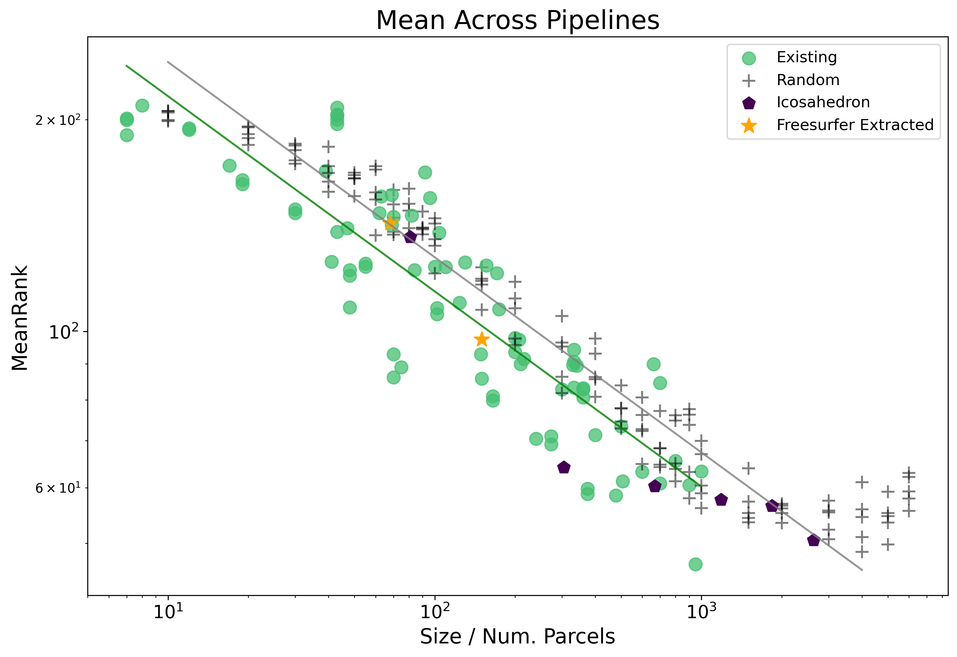
Is it problematic that we only have random parcellations with over 3,000 parcels? No, but see here for a more detailed look.
An additional page recreating this results according to Alternative Ranks is also provided here.
We can also alternately model parcellation type as as both a fixed effect and with a possible interaction with Size.
{% include base_results2.html %}
We see that in this case none of the interactions with Size are significant.
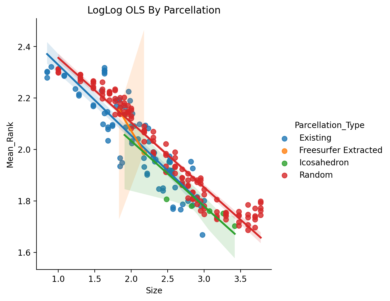
Plotting the basic fits by parcellation type we can see that for parcellations types with only a few samples it is difficult to conclude anything as the sample size is not sufficient.
A key point of interest beyond comparing between parcellation type is the coef. for Size. This represents the scaling exponent in a powerlaw relationship between Size and Performance. We see that despite the choice of how we model parcellation type, this estimated coef. stays fairly stable. Lastly, exploring the interactive plot may be useful seeing how any one parcellation did.
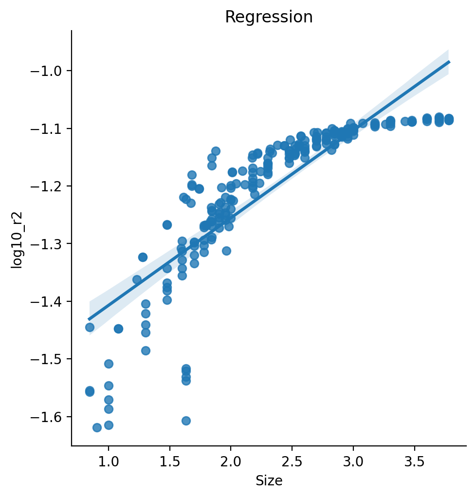
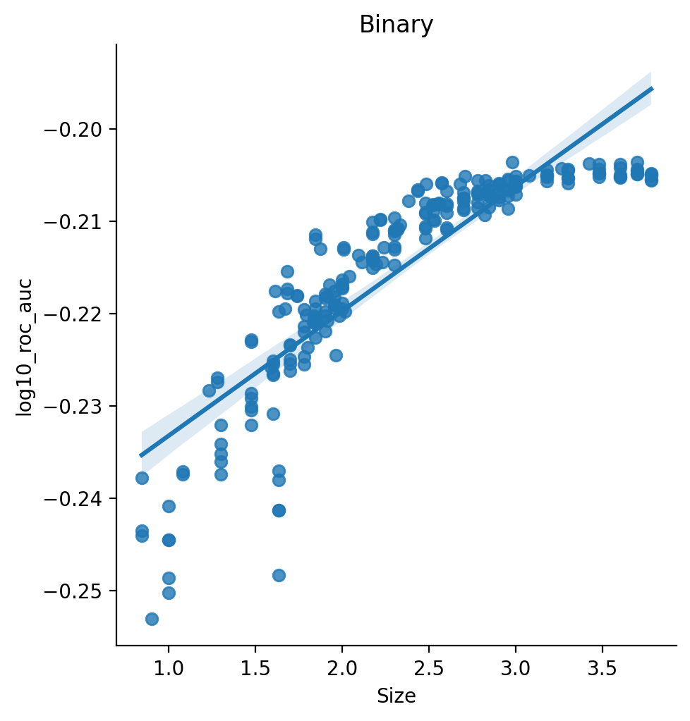
What happens when we look at the results separately for regression and binary targets, according to their respective raw metrics? Note that because we are limiting each analyses to one problem type, the results shown are averaged over less target variables (22 / 23).
Keep in mind also when interpreting the below results that it is fundamentally flawed to look at the raw metrics directly! These results should therefore not be considered as standalone results, see Mean Rank for a description on why this occurs.
An Interactive plot by parcellation type as plotted according to R2 values can be found here.
{% include base_results1_r2.html %}
An Interactive plot by parcellation type as plotted according to ROC AUC values can be found here.
{% include base_results1_roc_auc.html %}
The table below includes all parcellations specific scores. Notably these are mean relative rankings as averaged across both target variables and ML pipelines. Mean R2 and ROC AUC are calculated only from their relevant subsets of 22 and 23 target variables respectively. Warning: Mean R2 and ROC AUC should be taken with a grain of salt due to scaling issues between different targets.
Table columns are sortable! {: style="font-size: 85%; text-align: center;"}
{% include raw_results1.html %}