import sys
sys.path.append('/home/paperspace/repos/fastai/')
# !wget http://files.grouplens.org/datasets/movielens/ml-latest-small.zip# !unzip ml-latest-small.zip%reload_ext autoreload
%autoreload 2
%matplotlib inline
import torch
from fastai.learner import *
from fastai.column_data import *path='ml-latest-small/'ratings = pd.read_csv(path+'ratings.csv')
ratings.head().dataframe tbody tr th {
vertical-align: top;
}
.dataframe thead th {
text-align: right;
}
| userId | movieId | rating | timestamp | |
|---|---|---|---|---|
| 0 | 1 | 31 | 2.5 | 1260759144 |
| 1 | 1 | 1029 | 3.0 | 1260759179 |
| 2 | 1 | 1061 | 3.0 | 1260759182 |
| 3 | 1 | 1129 | 2.0 | 1260759185 |
| 4 | 1 | 1172 | 4.0 | 1260759205 |
movies = pd.read_csv(path+'movies.csv')
movies.head().dataframe tbody tr th {
vertical-align: top;
}
.dataframe thead th {
text-align: right;
}
| movieId | title | genres | |
|---|---|---|---|
| 0 | 1 | Toy Story (1995) | Adventure|Animation|Children|Comedy|Fantasy |
| 1 | 2 | Jumanji (1995) | Adventure|Children|Fantasy |
| 2 | 3 | Grumpier Old Men (1995) | Comedy|Romance |
| 3 | 4 | Waiting to Exhale (1995) | Comedy|Drama|Romance |
| 4 | 5 | Father of the Bride Part II (1995) | Comedy |
We create a crosstab of the most popular movies and most movie-addicted users which we'll copy into Excel for creating a simple example. This isn't necessary for any of the modeling below however.
g=ratings.groupby('userId')['rating'].count()
topUsers=g.sort_values(ascending=False)[:15]

g=ratings.groupby('movieId')['rating'].count()
topMovies=g.sort_values(ascending=False)[:15]

top_r = ratings.join(topUsers, rsuffix='_r', how='inner', on='userId')
top_r = top_r.join(topMovies, rsuffix='_r', how='inner', on='movieId')

#pd.crosstab(top_r.userId, top_r.movieId, top_r.rating, aggfunc=np.sum)Note that windows Office has add-ins. You can turn on the "solver" in the add-ins. This will run an iterative solver
wd- L2 regularizationn_factors- embedding sizes
val_idxs = get_cv_idxs(len(ratings))
wd=2e-4
n_factors = 50ratings.csvuserIdmovieIdrating- dependent variable
This movie and user, which other movies are similar to it, which people are similar to this person?
cf = CollabFilterDataset.from_csv(path, 'ratings.csv', 'userId', 'movieId', 'rating')- size embedding
- index
- batch size
- which optimizer
learn = cf.get_learner(n_factors, val_idxs, 64, opt_fn=optim.Adam)learn.fit(1e-2, 2, wds=wd, cycle_len=1, cycle_mult=2)Failed to display Jupyter Widget of type HBox.
If you're reading this message in the Jupyter Notebook or JupyterLab Notebook, it may mean that the widgets JavaScript is still loading. If this message persists, it likely means that the widgets JavaScript library is either not installed or not enabled. See the Jupyter Widgets Documentation for setup instructions.
If you're reading this message in another frontend (for example, a static rendering on GitHub or NBViewer), it may mean that your frontend doesn't currently support widgets.
[ 0.       0.84641  0.80873]
[ 1.       0.78206  0.77714]
[ 2.       0.5983   0.76338]
math.sqrt(0.776)0.8809086218218096
preds = learn.predict()y=learn.data.val_y[:,0]
sns.jointplot(preds, y, kind='hex', stat_func=None);

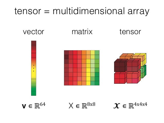
T = tensor in Torch
a = T([[1.,2],[3,4]])
b = T([[2.,2],[10,10]])
a,b
(
1 2
3 4
[torch.FloatTensor of size 2x2],
2 2
10 10
[torch.FloatTensor of size 2x2])
a*b 2 4
30 40
[torch.FloatTensor of size 2x2]
(a*b).sum(1) 6
70
[torch.FloatTensor of size 2]
We are extending the nn.Module from pytorch
forward is a inherited method from the nn.Module, which is leveraged by other functions in other pytorch libraries
forward<- matrix multiplicationbackwards<- gradients
class DotProduct(nn.Module):
def forward(self, u, m): return (u*m).sum(1)model=DotProduct()model(a,b) 6
70
[torch.FloatTensor of size 2]
- look at unique values of user_ids
- make a mapping from user_id to a INT (so there's no skipping of numbers)
- do the same for movie ids
enumerate- takes in a collection, gives back the index, value for a collectionlambda- python keyword for making a temporary function
u_uniq = ratings.userId.unique()
user2idx = {o:i for i,o in enumerate(u_uniq)}
ratings.userId = ratings.userId.apply(lambda x: user2idx[x])

m_uniq = ratings.movieId.unique()
movie2idx = {o:i for i,o in enumerate(m_uniq)}
ratings.movieId = ratings.movieId.apply(lambda x: movie2idx[x])

n_users=int(ratings.userId.nunique())
n_movies=int(ratings.movieId.nunique())-
__init__- this function is called when the object is created. Called the constructor -
obj = myClass()
-
obj = newClassImade(list)
-
nn.Embedding- a pytorch object -
self.u.weight.data- initializing the user weights to a reasonable starting place -
self.m.weight.data- initializing the movie weights to a reasonable starting place -
uniform_- note that_means 'inplace' instead of returning a variable and doing an assignment
- users,movies = cats[:,0],cats[:,1]
he is pulling both datasets out of the categorical variable.
class EmbeddingDot(nn.Module):
    def __init__(self, n_users, n_movies):
        super().__init__()
        self.u = nn.Embedding(n_users, n_factors)
        self.m = nn.Embedding(n_movies, n_factors)
        self.u.weight.data.uniform_(0,0.05)
        self.m.weight.data.uniform_(0,0.05)

    def forward(self, cats, conts):
        users,movies = cats[:,0],cats[:,1]
        u,m = self.u(users),self.m(movies)
return (u*m).sum(1)x = ratings.drop(['rating', 'timestamp'],axis=1)
y = ratings['rating']data = ColumnarModelData.from_data_frame(path, val_idxs, x, y, ['userId', 'movieId'], 64)optim- gives us an optimizer.model.parameters()this is inherited from thenn.Module.1e-1- is the learning rateweight decay- regularizationmomentum
wd=1e-5
model = EmbeddingDot(n_users, n_movies).cuda()
opt = optim.SGD(model.parameters(), 1e-1, weight_decay=wd, momentum=0.9)fit(model, data, 3, opt, F.mse_loss)Failed to display Jupyter Widget of type HBox.
If you're reading this message in the Jupyter Notebook or JupyterLab Notebook, it may mean that the widgets JavaScript is still loading. If this message persists, it likely means that the widgets JavaScript library is either not installed or not enabled. See the Jupyter Widgets Documentation for setup instructions.
If you're reading this message in another frontend (for example, a static rendering on GitHub or NBViewer), it may mean that your frontend doesn't currently support widgets.
[ 0.       1.68932  1.64501]
[ 1.       1.08445  1.30609]
[ 2.       0.91446  1.23001]
### Set the learning rateset_lrs(opt, 0.01)fit(model, data, 3, opt, F.mse_loss)Failed to display Jupyter Widget of type HBox.
If you're reading this message in the Jupyter Notebook or JupyterLab Notebook, it may mean that the widgets JavaScript is still loading. If this message persists, it likely means that the widgets JavaScript library is either not installed or not enabled. See the Jupyter Widgets Documentation for setup instructions.
If you're reading this message in another frontend (for example, a static rendering on GitHub or NBViewer), it may mean that your frontend doesn't currently support widgets.
[ 0.       0.69273  1.14723]
[ 1.       0.72746  1.1352 ]
[ 2.       0.67176  1.12943]
min_rating,max_rating = ratings.rating.min(),ratings.rating.max()
min_rating,max_rating
(0.5, 5.0)
With the sigmoid function we can multiply by our target range
F - its the pytorch functional. its a large library of functions used in deep learning
def get_emb(ni,nf):
    e = nn.Embedding(ni, nf)
    e.weight.data.uniform_(-0.01,0.01)
    return e

class EmbeddingDotBias(nn.Module):
    def __init__(self, n_users, n_movies):
        super().__init__()
        (self.u, self.m, self.ub, self.mb) = [get_emb(*o) for o in [
            (n_users, n_factors), (n_movies, n_factors), (n_users,1), (n_movies,1)
        ]]

    def forward(self, cats, conts):
        users,movies = cats[:,0],cats[:,1]
        um = self.u(users)* self.m(movies)

        ## add in user bias and movie bias
        ## squeeze is going to be broadcasting, this will replicate a vector
        ## and add it to the matrix
        res = um.sum(1) + self.ub(users).squeeze() + self.mb(movies).squeeze()

        ## this limits the range of the ratings
        res = F.sigmoid(res) * (max_rating-min_rating) + min_rating
return reswd=2e-4
model = EmbeddingDotBias(cf.n_users, cf.n_items).cuda()
opt = optim.SGD(model.parameters(), 1e-1, weight_decay=wd, momentum=0.9)fit(model, data, 3, opt, F.mse_loss)Failed to display Jupyter Widget of type HBox.
If you're reading this message in the Jupyter Notebook or JupyterLab Notebook, it may mean that the widgets JavaScript is still loading. If this message persists, it likely means that the widgets JavaScript library is either not installed or not enabled. See the Jupyter Widgets Documentation for setup instructions.
If you're reading this message in another frontend (for example, a static rendering on GitHub or NBViewer), it may mean that your frontend doesn't currently support widgets.
[ 0.       0.85056  0.83742]
[ 1.       0.79628  0.81775]
[ 2.       0.8012   0.80994]
def get_emb(ni,nf):
    e = nn.Embedding(ni, nf)
    e.weight.data.uniform_(-0.05,0.05)
    return e

class EmbeddingDotBias(nn.Module):
    def __init__(self, n_factors, n_users, n_items, min_score, max_score):
        super().__init__()
        self.min_score,self.max_score = min_score,max_score
        (self.u, self.i, self.ub, self.ib) = [get_emb(*o) for o in [
            (n_users, n_factors), (n_items, n_factors), (n_users,1), (n_items,1)
        ]]

    def forward(self, users, items):
        um = self.u(users)* self.i(items)
        res = um.sum(1) + self.ub(users).squeeze() + self.ib(items).squeeze()
        return F.sigmoid(res) * (self.max_score-self.min_score) + self.min_score
Let's look at the excel
All the users are compared to all movies
(self.u, self.m) = [get_emb(*o) for o in..create embeddingsnn.Linear(n_factors*2, 10, nh)- create our linear layersnhnumber of hidden layerstorch.cat([self.u(users),self.m(movies)], dim=1)adds the two users and movies togetherF.relu(self.lin1(x)- linear
- relu 0, or Max; truncates negative values
- we have 1 layer, it is a NN, maybe not 'deep' per say
class EmbeddingNet(nn.Module):
    def __init__(self, n_users, n_movies, nh=10):
        super().__init__()
        (self.u, self.m) = [get_emb(*o) for o in [
            (n_users, n_factors), (n_movies, n_factors)]]
        self.lin1 = nn.Linear(n_factors*2, 10, nh)
        self.lin2 = nn.Linear(10, 1)

    def forward(self, cats, conts):
        users,movies = cats[:,0],cats[:,1]
        x = F.dropout(torch.cat([self.u(users),self.m(movies)], dim=1), 0.75)
        x = F.dropout(F.relu(self.lin1(x)), 0.75)
return F.sigmoid(self.lin2(x)) * (max_rating-min_rating+1) + min_rating-0.5wd=5e-4
model = EmbeddingNet(n_users, n_movies).cuda()
opt = optim.SGD(model.parameters(), 1e-2, weight_decay=wd, momentum=0.9)fit(model, data, 3, opt, F.mse_loss)Failed to display Jupyter Widget of type HBox.
If you're reading this message in the Jupyter Notebook or JupyterLab Notebook, it may mean that the widgets JavaScript is still loading. If this message persists, it likely means that the widgets JavaScript library is either not installed or not enabled. See the Jupyter Widgets Documentation for setup instructions.
If you're reading this message in another frontend (for example, a static rendering on GitHub or NBViewer), it may mean that your frontend doesn't currently support widgets.
[ 0.       1.0879   1.10568]
[ 1.       0.81337  0.82665]
[ 2.       0.80449  0.79857]
set_lrs(opt, 1e-3)fit(model, data, 3, opt, F.mse_loss)Failed to display Jupyter Widget of type HBox.
If you're reading this message in the Jupyter Notebook or JupyterLab Notebook, it may mean that the widgets JavaScript is still loading. If this message persists, it likely means that the widgets JavaScript library is either not installed or not enabled. See the Jupyter Widgets Documentation for setup instructions.
If you're reading this message in another frontend (for example, a static rendering on GitHub or NBViewer), it may mean that your frontend doesn't currently support widgets.
[ 0.       0.68968  0.79054]
[ 1.       0.71873  0.78805]
[ 2.       0.70101  0.78719]
- We can add dropouts
- we can use embeddings of different sizes
- we can add more hidden layers with more nodes
- we can add different amounts of regularization
What's happening inside? - opt = optim.SGD(model.parameters(), 1e-2, weight_decay=wd, momentum=0.9)


- 1,000,000 ---> trasnformation ---> 100k
When you have a high dimensional space, yoru gradient becomes a huge matrix. The amount of calculation computation that you need is very high. Takes up a lot of memory, a lot of time.
Look up :
- jacobian
- hessian
More efficient -> find the derivatives analytically instead of finite differencing
Explaining the manual calculation of the differentials, ot calculate a new a and b (orange), then run all back again
- looking at SGD de/da, we see that it is positive and negative at random
- the momentum idea is controlled by beta coefficients, will keep the differential going in the same direction, but a bit faster; will reduce the number of iterations
- adam is much much faster, but the answers are not as good as SGD with momentum
- Recently, a newer version is out: adamW that fixes weight decay issues. Ideally this will be fixed going forward
Equals to our previous value of b, times learning rate divided by sqrt()
cellJ8= linear interpolation of derivative and the previous directioncellL8= linear interpolation of derivative squared + derivative squared from last step- this is also known as exponential weighted moving average
- squared derivative is always positive
- if there's a big change, the squared derivative will be huge
- so if there's a big change, we divide the learning rate by a big number, (slow down)
- if there's minimal change ( we will be more aggressive in choosing a new learning rate)
- adaptive learning rate - since the rate isn't constant, but dependent the model's optimization movements
avg_loss = avg_loss * avg_mom + loss * (1-avg_mom)From the fit function:
def fit(model, data, epochs, opt, crit, metrics=None, callbacks=None, **kwargs):
    """ Fits a model
    Arguments:
       model (model): any pytorch module
           net = to_gpu(net)
       data (ModelData): see ModelData class and subclasses
       opt: optimizer. Example: opt=optim.Adam(net.parameters())
       epochs(int): number of epochs
       crit: loss function to optimize. Example: F.cross_entropy
    """
    stepper = Stepper(model, opt, crit, **kwargs)
    metrics = metrics or []
    callbacks = callbacks or []
    avg_mom=0.98
    batch_num,avg_loss=0,0.

    for epoch in tnrange(epochs, desc='Epoch'):
        stepper.reset(True)
        t = tqdm(iter(data.trn_dl), leave=False, total=len(data.trn_dl))
        for (*x,y) in t:
            batch_num += 1
            loss = stepper.step(V(x),V(y))

            avg_loss = avg_loss * avg_mom + loss * (1-avg_mom) #<----------

            debias_loss = avg_loss / (1 - avg_mom**batch_num)
            t.set_postfix(loss=debias_loss)
            stop=False
            for cb in callbacks: stop = stop or cb.on_batch_end(debias_loss)
            if stop: return

        vals = validate(stepper, data.val_dl, metrics)
        print(np.round([epoch, debias_loss] + vals, 6))
        stop=False
        for cb in callbacks: stop = stop or cb.on_epoch_end(vals)
        if stop: break