-
Notifications
You must be signed in to change notification settings - Fork 9
Use cases
The problem is related to the identification of the Youngs modulus of concrete from experimental tests. It includes multiple levels
- Identification using the procedure from the standard - take the third loading cycle and chose a (random) reading before and after the loading (within the 20s) and compute the secant modulus (this is the Young's modulus)
- include the data during the loading phase as well
- include the uncertainty of the measurements (including both stress/strain or similarly load/displacements)
- estimate, how good the model is able to approximate the first and second loading cycle as well as the third one
- assume that for each sample (e.g. usually 3, but we usually have the compression data = first cycle for another 3) there is a different Young's modulus, compute the distribution of these Youngs moduli
- use an elastic model with the parameters identified from above in a constitutive formulation to predict the probability distribution of the mid-span displacement of a structure (e.g. 3-point bending test)


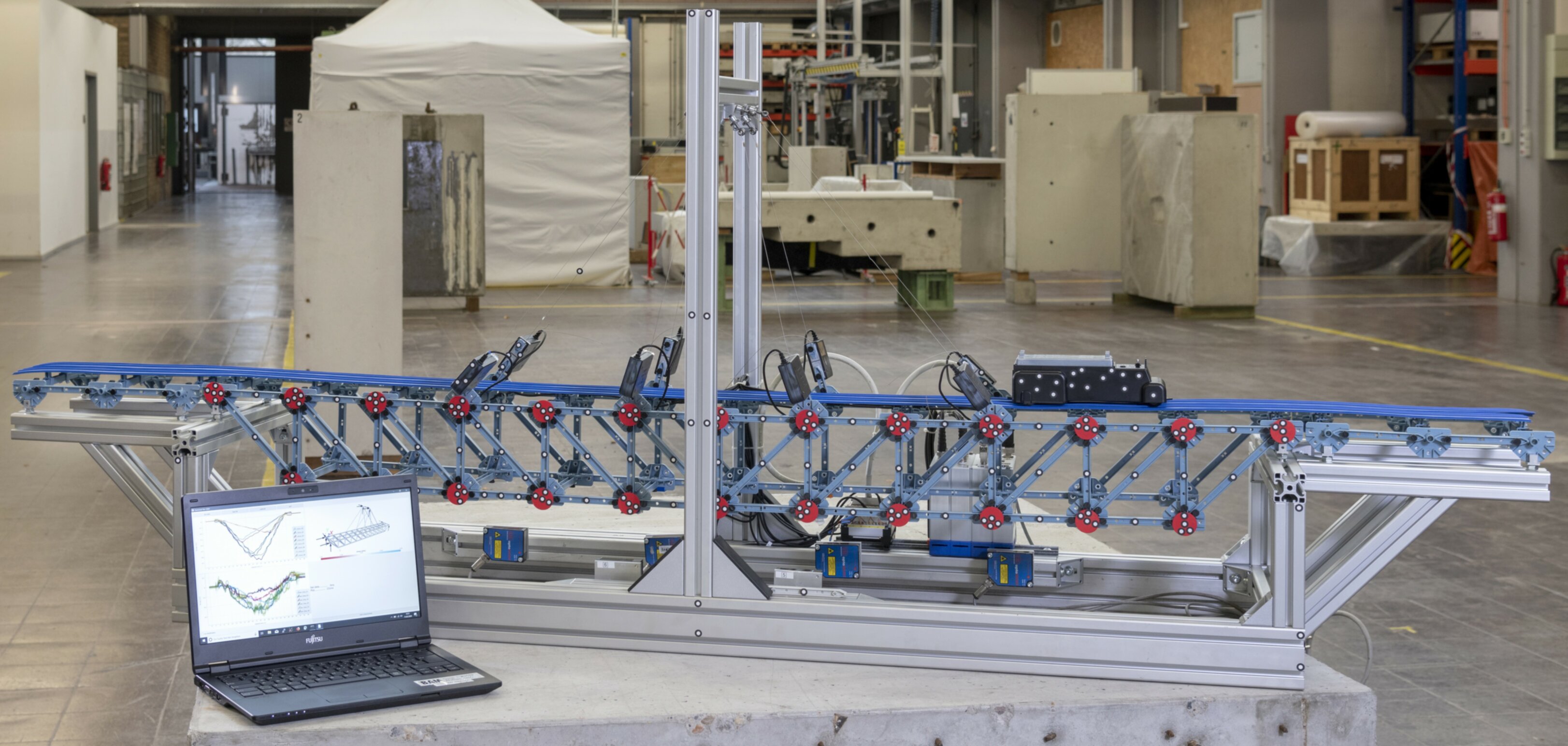
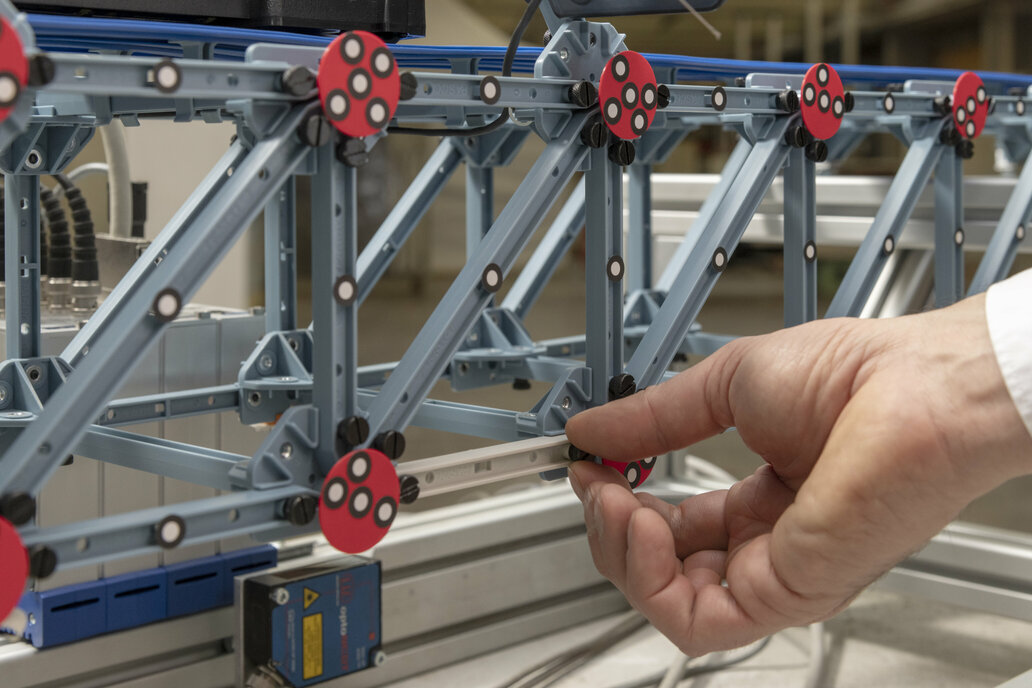
The setup is used to illustrate the concept of a digital twin. Here, additional information should be provided by augmenting data with models to predict data that is not measurable (in this case that could be a stress within the structure, e.g. for a fatigue analysis). In the setting, we are continously measuring the forces in 8 cables, the vertical displacement at 6 positions using laser sensors (10Hz) and additionally stereo cameras measuring displacements at the disk with the dots as seen in the figure. The latter is a different measuring device with a separate data acquisition system.
- The first question is to understand what a good model is (2D/3D, trusses/beams/beams with connections).
- Then, it is important to understand, where the model is "wrong" and potentially how to improve it.
- The goal in realtime is to identify while the car is passing over the bridge information related to its position, the speed.
- Finally, it is interesting to analyze the probability of failure, e.g. the probability the stress (not measured but an output of the bridge FEM model) is larger than a certain threshold.
Given insitu-CT data (complete displacement field) in a compression test or 3 point bending test for different loading scenarios, identify the constitutive model and also regions in the stress-strain domain that are not accurately captured by the model. Use the approach of the displacements in the model being latent random variables (FEMU-F) with the likelihood function being the residual of the pde to be solved. This can potentially be extended to multiple specimens (identifying a distribution of parameters instead of a single set of parameters).
This problem deals with finding the probability distribution of a threshold value that cannot be measured directly. As a result we will have to deal with censored data. Assume you produce an explosive (say sticks of dynamite) and you want to know to know the critical height from which you can drop a stick of dynamite triggering its explosion. Since you are a practical person, you conduct several tests (each time with a new stick of dynamite) where you drop the sticks from different heights (usually one applies so-called staircase or up-and-down test schemes here, see https://en.wikipedia.org/wiki/Up-and-Down_Designs). The outcome of each test is always one of two things: either you get an explosion or or you don't. After all experiments have been conducted, you want to estimate the probability density function (PDF) of the critical height, since you consider the critical height as a random variable across your produced sticks of dynamite.
Let us assume that the unknown distribution of the critical height - let us call it - follows a normal distribution
. Hence, we want to infer the two parameters
and
. In order to formulate the likelihood function let us think about what each experiment tells us about
. First, let us assume that each stick of dynamite has its own "true" critical height. If we let it fall from a height lower than its true critical height, it will not explode and if we let it drop from a greater (or equal) elevation than its true critical height it will explode. So, if an experiment results in an explosion, we infer that the critical height of that particular stick was smaller or equal to the tested elevation, however, we do not know the exact value. This can be interpreted as a left-censored data point. Conversely, if an experiment does not result in an explosion we can conclude that the critical height of the corresponding stick was greater than the tested elevation - hence we have a right-censored data point. The corresponding likelihood function looks like this:
Here, is the parameter vector,
is the number of conducted tests,
and
are the tested elevation and the true critical height of dynamite stick
respectively, and
is defined as 1 if test
resulted in an explosion, and
if no explosion occurred in test
. If we replace the general terms
with the respective ones of the normal distribution, we obtain
where is the cumulative distribution function (CDF) of the standard normal distribution. Given some test data, one can now solve this problem in a frequentist manner by maximizing the likelihood, or via a Bayesian approach, if one additionally defines priors for
and
.
Assume you are the manufacturer of some mechanical component, whose structural integrity is import for safety reasons. Further assume, that the considered component is primarily experiencing cyclic loads during operation (the maginitude of which is known), so that the most important failure mode to design against is fatigue (e.g. low cycle faituge, LCF). In this setup, you now want to estimate the expected life of your component in statistical terms, so that you can give some guarantees about the component life span. Since the component is relevant from a safety perspective, you decide to do direct component testing. So, you take components from your production line, and give it to your testing lab. Since the testing procedure is expensive, you decide that each experiment should be stoped if failure did not occurr when reaching a high number of cycles, let us call it
.
The component life span is modeled as a random variable with a Weibull distribution, i.e.
with scale
and shape
. From the
tested components most of them failed before reaching
, but some were still intact when reaching
. The latter components are called runouts, and they represent right-censored data points, since their life is only specified to being greater than
. The likelihood of this problem reads
where is the parameter vector,
is the number of applied load cycles on component
until failure occurred, or
was reached,
is the probability density function (PDF) of the Weibull distribution and
is a flag with
if component
failed during the test, and
if component
was a runout. If we express the general terms in the above equation with the PDF and CDF of the Weibull distribution, we obtain
Given the results of the test campaign - similar to the usecase presented before - a parameter estimation can be obtained via the maximum likelihood method (frequentist approach), or via a Bayesian framework once priors for and
are defined.
Latex modeling with hack for latex rendering
Here is some text related to likelihood and prior, forward model, data, ..
Here is some text related to the approach used to solve the problem (Gibbs, MCMC, special structures)