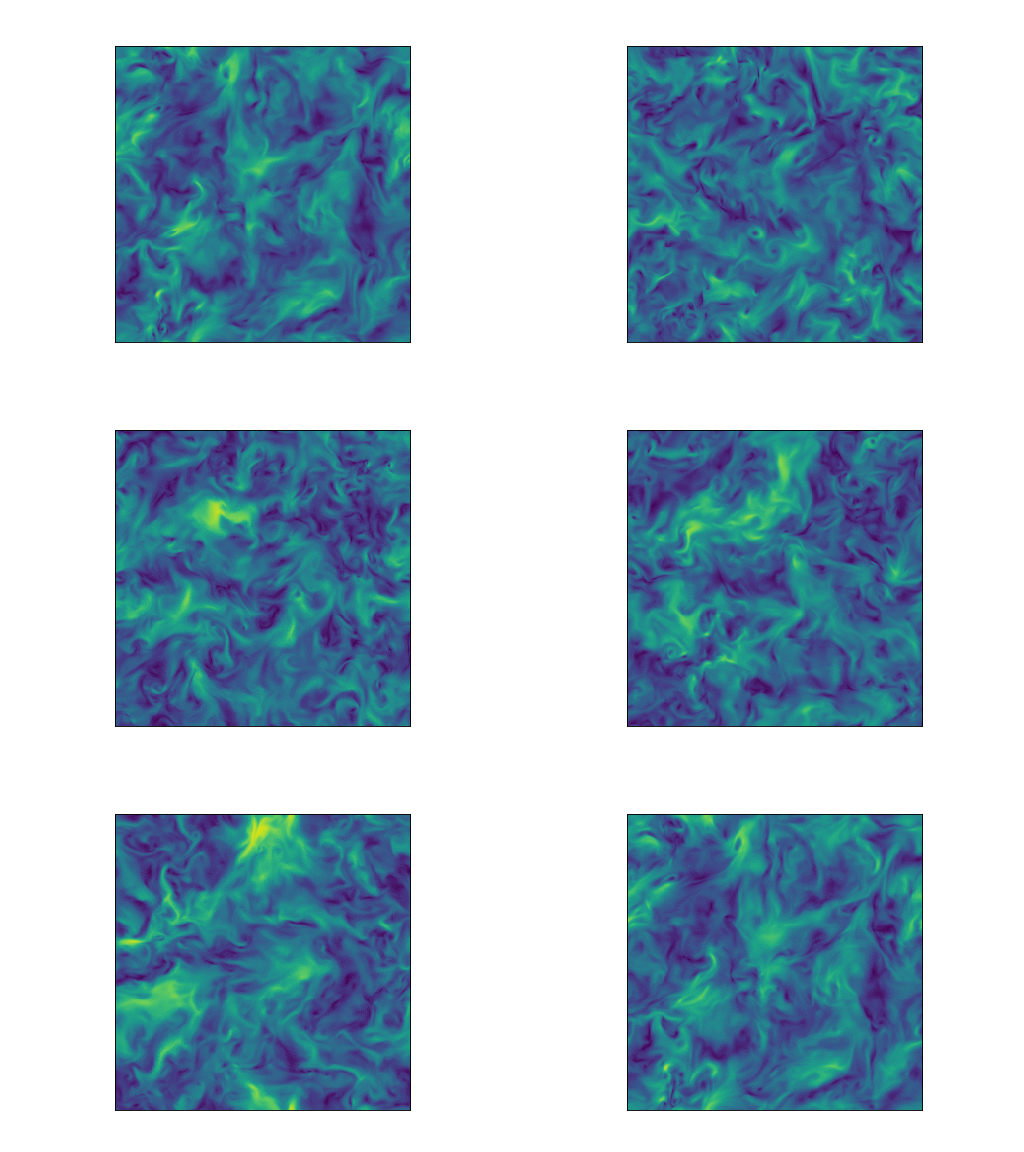
Isotropic turbulence with Re_lambda=128 computed using the NS solver and a mesh of size 300**3 is physical space.
spectralDNS contains a classical high-performance pseudo-spectral Navier-Stokes DNS solver for triply periodic domains. The most notable feature of this solver is that it's written entirely in Python using NumPy, MPI for Python (mpi4py) and pyFFTW. MPI decomposition is performed using either the "slab" or the "pencil" approach and, stripping away unnecessary pre- and post-processing steps, the slab solver is no more than 100 lines long, including the MPI. The code has been found to scale very well in tests on the Shaheen Blue Gene/P supercomputer at KAUST Supercomputing Laboratory. Results of both weak and strong scaling tests are shown below. In addition to incompressible Navier-Stokes there are also solvers for MHD and Navier-Stokes or MHD with variable density through a Boussinesq approximation. The solver is described more thoroughly in this paper:
M. Mortensen and H. P. Langtangen "High performance Python for direct numerical simulations of turbulent flows", Computer Physics Communications 203, p 53-65 (2016) http://arxiv.org/pdf/1602.03638v1.pdf
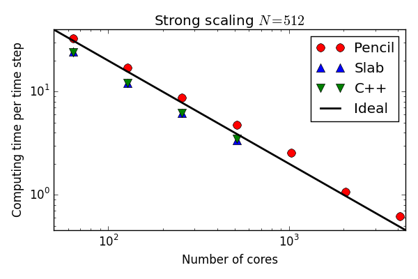
The efficiency of the pure NumPy/mpi4py solver has been enhanced using Cython for certain routines. The strong scaling results on Shaheen shown below have used the optimized Python/Cython solver, which is found to be faster than a pure C++ implementation of the same solver.
A channel flow solver is implemented using the Shen basis (Jie Shen, SIAM Journal on Scientific Computing, 16, 74-87, 1995) for the scheme described by Kim, Moin and Moser (J. Fluid Mechanics, Vol 177, 133-166, 1987). The solver is described here: https://arxiv.org/pdf/1701.03787v1.pdf
spectralDNS contains a setup.py script and can be installed by cloning or forking the repository and then with regular python distutils
python setup.py install --prefix="path used for installation. Must be on the PYTHONPATH"
or in-place using
python setup.py build_ext --inplace
However, spectralDNS depends on two other modules in the spectralDNS organization: shenfun and mpi4py-fft. And besides that, it requires h5py built with parallel HDF5, for visualizing the results, and cython, numba or pythran are used to optimize a few routines. These dependencies are all available on conda forge and a proper environment would be
conda create --name spectralDNS -c conda-forge shenfun mpi4py-fft cython numba pythran mpich pip h5py=*=mpi*
conda activate spectralDNS
Furthermore, you may want to use matplotlib for plotting and nodepy is used for some of the integrators. The latter should be installed using pypi
pip install nodepy
Another possibility is to compile spectralDNS yourselves using conda build. From the main directory after forking or cloning do, e.g.,
conda build -c conda-forge conf/conda
conda install spectralDNS --use-local
which will also build and install the required dependencies.
If you do not use conda, then the dependencies must be installed through other channels. Both shenfun and mpi4py-fft can be installed using pypi
pip install shenfun
pip install mpi4py-fft
But note that these require MPI for Python and serial FFTW libraries. See further installation instructions.
See the demo folder for extensive usage.
There are different solvers. For example, there are two Navier Stokes solvers for the triply periodic domain. A regular one (solvers/NS.py), and one based on a velocity-vorticity formulation (solvers/VV.py). The solver of your choice is required as an argument when running:
cd demo
mpirun -np 4 python TG.py NS
or
mpirun -np 4 python TG.py VV
There are many different arguments to each solver. They are all described in config.py. Arguments may be specified on the commandline
mpirun -np 4 python TG.py --M 6 6 6 --precision single --dealias '3/2-rule' NS
before the required solver argument. Alternatively, use config.update as shown in demo/TG.py.
To visualize the generated data you can do
from mpi4py_fft import generate_xdmf
generate_xdmf('name of h5-file')
and then open the generated xdmf-file in Paraview. Note that generate_xdmf must be run on only one single processor.
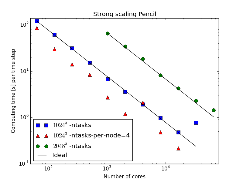
The most recent simulations of the pencil version of the NS solver are showing excellent scaling up to 65k cores at KAUST and Shaheen II!
The difference between the red triangles and the blue squares are simply the number of mpi processes sent to each node on Shaheen II. The default version (blue squares) are filling up all nodes with 32 processes on each, whereas the red triangles have only four processes for each node. The green dots have been sampled using the default settings.Results also from the old Shaheen BlueGene/P:
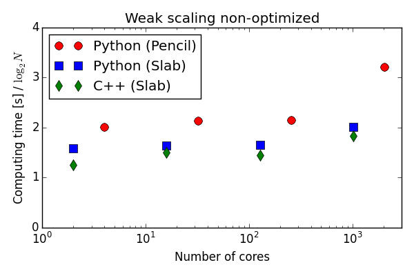
Weak scaling of pure numpy/mpi4py solver on Shaheen BlueGene/P. The C++ solver uses slab decomposition and MPI communication is performed by the FFTW library.
Strong scaling of optimized Python/Cython solver on Shaheen BlueGene/P. The C++ solver uses slab decomposition and MPI communication is performed by the FFTW library.
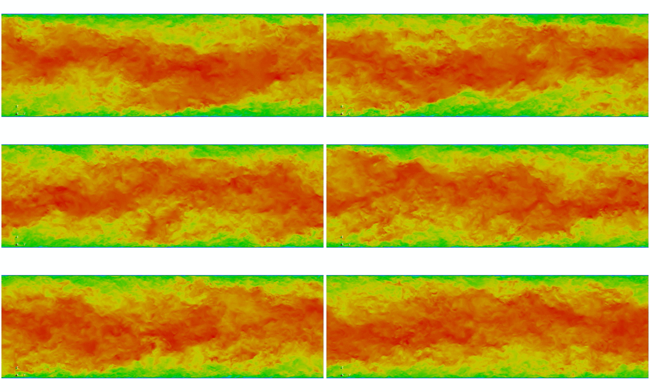
Turbulent channel flow at Re_tau = 2000. Simulations are performed using 512 cores on Shaheen II with the KMM channel flow solver (solvers/KMM.py) using 512x1024x1024 points in real physical space.
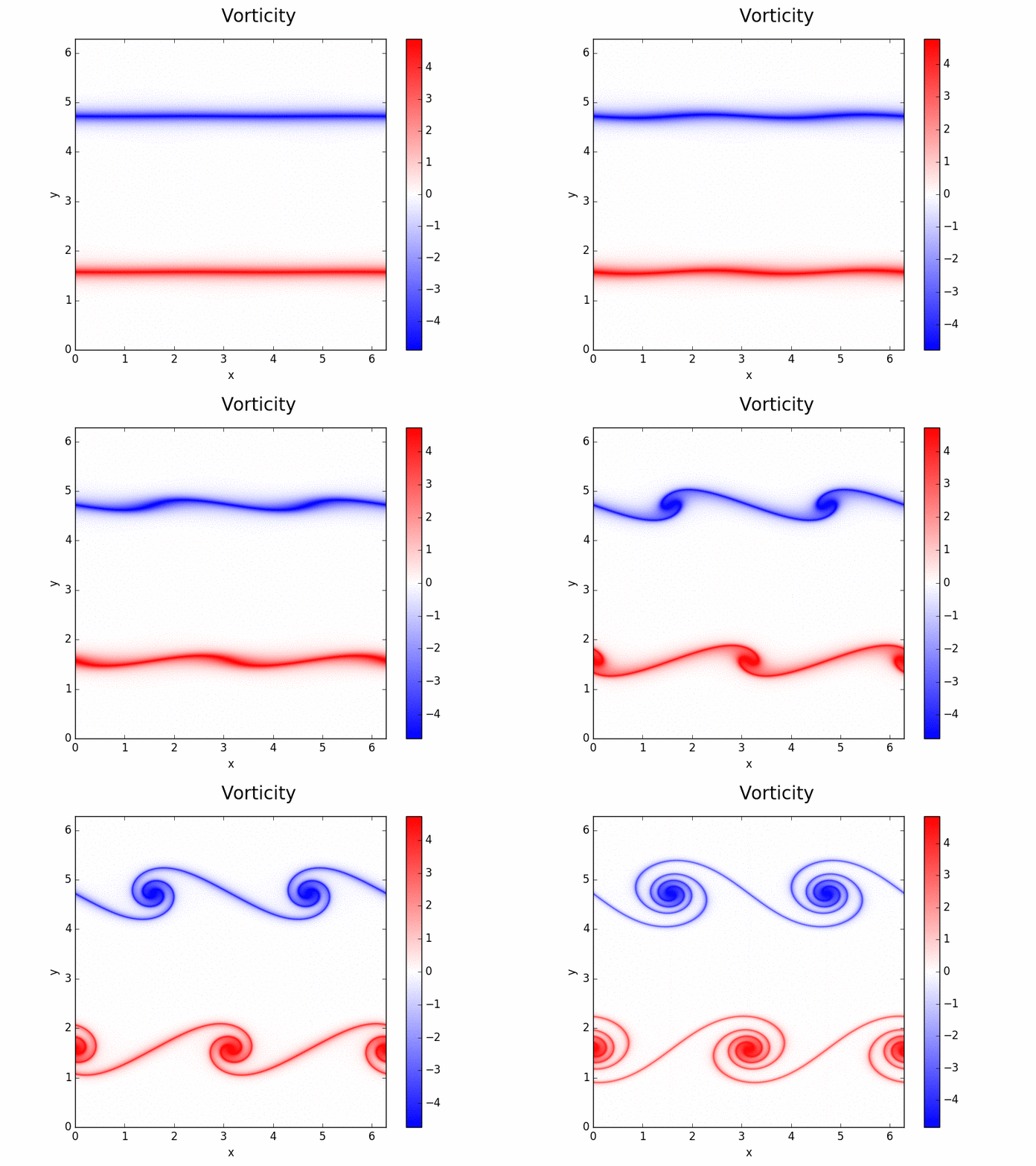
Evolution of vorticity. Two-dimensional simulation of Kelvin Helmholtz shear instability using a 2D solver (solvers/NS2D.py)
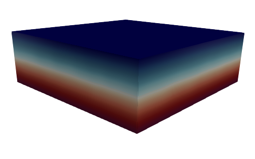
Turbulent Rayleigh-Bénard flow computed with the KMMRK3_RB solver (solvers/KMMRK3_RB.py) using 512x512x256 points in real physical space. Shown is the concentration of a scalar with boundary condition 0 and 1 for the top and bottom, respectively. Note that the shown top lid is located just inside the wall, at z=0.991 (z domain is in [-1, 1]).
spectralDNS is developed by
- Mikael Mortensen
- Diako Darian
spectralDNS is licensed under the GNU GPL, version 3 or (at your option) any later version. spectralDNS is Copyright (2014-2020) by the authors.
The latest version of this software can be obtained from
https://github.com/spectralDNS/spectralDNS
Please report bugs and other issues through the issue tracker at:
