Mathematical modelling of infectious disease
Mathematical models can project how infectious diseases progress to show the likely outcome of an epidemic and help inform public health interventions. Models use basic assumptions or collected statistics along with mathematics to find parameters for various infectious diseases and use those parameters to calculate the effects of different interventions, like mass vaccination programmes. The modelling can help decide which intervention/s to avoid and which to trial, or can predict future growth patterns, etc. The basic reproduction number (denoted by R0) is a measure of how transferable a disease is. It is the average number of people that a single infectious person will infect over the course of their infection. This quantity determines whether the infection will spread exponentially, die out, or remain constant: if R0 > 1, then each person on average infects more than one other person so the disease will spread; if R0 < 1, then each person infects fewer than one person on average so the disease will die out; and if R0 = 1, then each person will infect on average exactly one other person, so the disease will become endemic: it will move throughout the population but not increase or decrease.
The basic reproduction number can be computed as a ratio of known rates over time: if an infectious individual contacts β other people per unit time, if all of those people are assumed to contract the disease, and if the disease has a mean infectious period of 1/γ, then the basic reproduction number is just R0 = β/γ. Some diseases have multiple possible latency periods, in which case the reproduction number for the disease overall is the sum of the reproduction number for each transition time into the disease. For example, Blower et al.[7] model two forms of tuberculosis infection: in the fast case, the symptoms show up immediately after exposure; in the slow case, the symptoms develop years after the initial exposure (endogenous reactivation). The overall reproduction number is the sum of the two forms of contraction: R0 = R0FAST + R0SLOW.
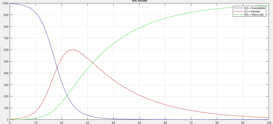
The SIR model divides the population in three groups:
S(t) is used to represent the individuals not yet infected with the disease at time t, or those susceptible to the disease of the population.
I(t) denotes the individuals of the population who have been infected with the disease and are capable of spreading the disease to those in the susceptible category.
R(t) is the compartment used for the individuals of the population who have been infected and then removed from the disease, either due to immunization or due to death. Those in this category are not able to be infected again or to transmit the infection to others.
Using a fixed population,N = S(t) + I(t) + R(t) in the three functions resolves that the value N should remain constant within the simulation. The model is started with values of S(t=0), I(t=0) and R(t=0). These are the number of people in the susceptible, infected and removed categories at time equals zero. Subsequently, the flow model updates the three variables for every time point with set values for β and γ . The simulation first updates the infected from the susceptible and then the removed category is updated from the infected category for the next time point (t=1). This describes the flow persons between the three categories. During an epidemic the susceptible category is not shifted with this model, β changes over the course of the epidemic and so does γ . These variables determine the length of the epidemic and would have to be updated with each cycle.
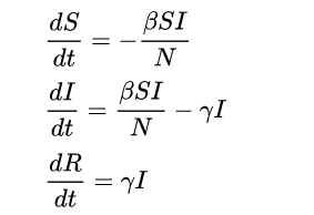
Several assumptions were made in the formulation of these equations: First, an individual in the population must be considered as having an equal probability as every other individual of contracting the disease with a rate of alpha and an equal number b of people that an individual makes contact with per unit time. Then, let β be the multiplication of alpha and b. This is the transmission probability times the contact rate. Besides, an infected individual makes contact with b persons per unit time whereas only a fraction, S/N of them are susceptible.Thus, we have every infective can infect abS/N -> βS/N susceptible persons,and therefore, the whole number of susceptibles infected by infectives per unit time is βS*I/N . For the second and third equations, consider the population leaving the susceptible class as equal to the number entering the infected class. However, a number equal to the fraction γ which represents the mean recovery/death rate, or 1 / γ the mean infective period) of infectives are leaving this class per unit time to enter the removed class. These processes which occur simultaneously are referred to as the Law of Mass Action, a widely accepted idea that the rate of contact between two groups in a population is proportional to the size of each of the groups concerned.Finally, it is assumed that the rate of infection and recovery is much faster than the time scale of births and deaths and therefore, these factors are ignored in this model.
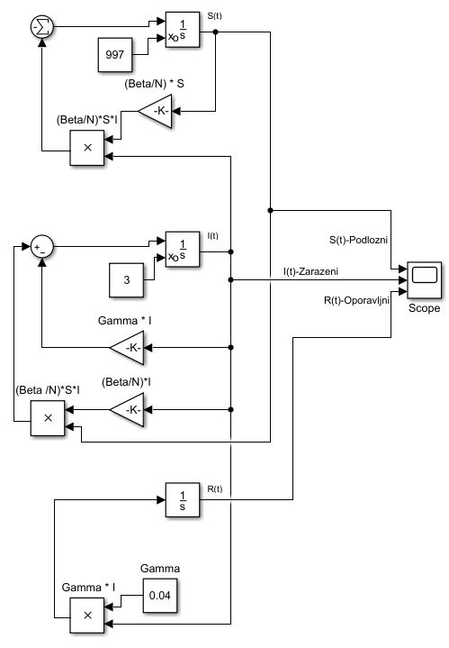
SIRmodel_Simulink.slx contains the solution of differential equations using MATLAB simulink so basic concept can be understood.
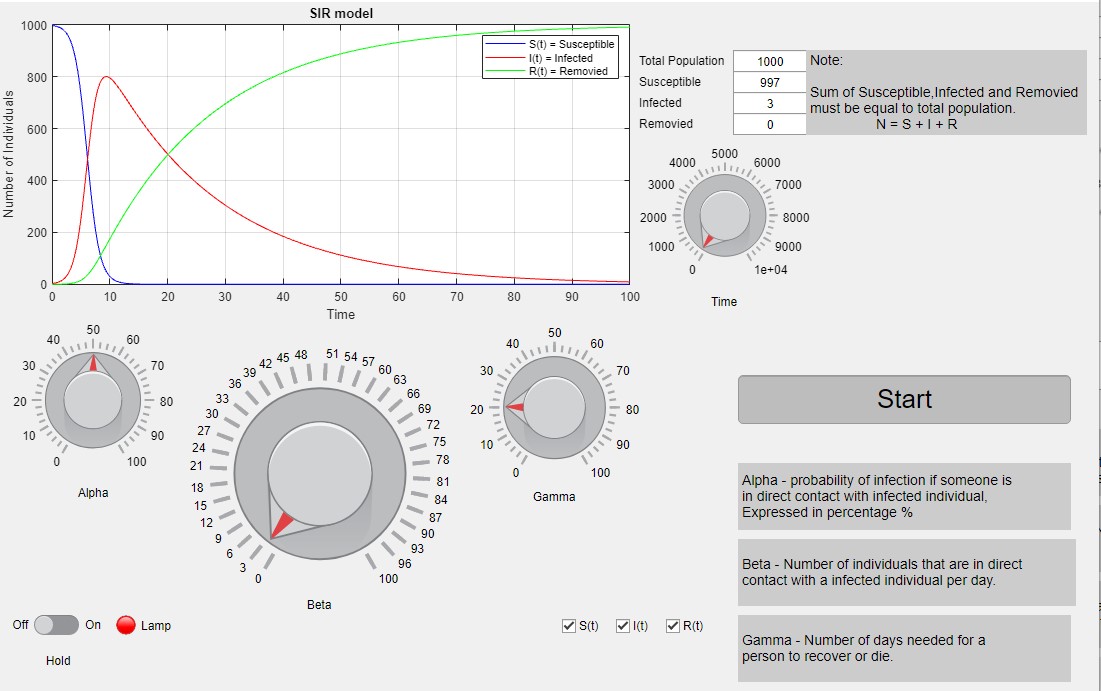
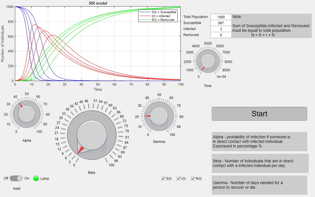
For changing the model parameters easily i made a MATLAB GUI so it's more straight forward process