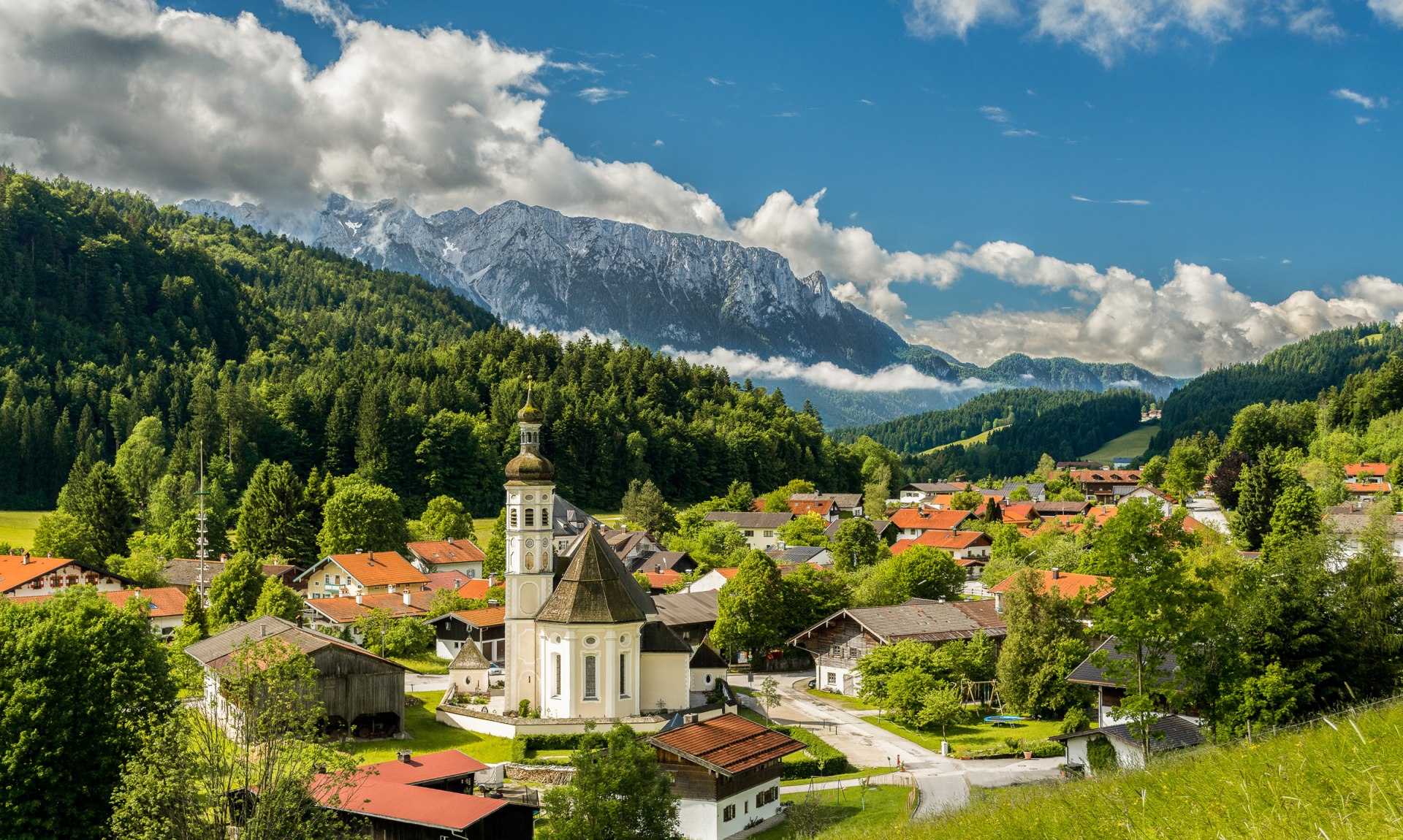
The project contains an exploratory remote sensing analysis of Sentinel-2 data over Sachrang, a small village in the Bavarian Alps.
It also reflects my personal connection to this area — it is idyllic in all seasons and hosts a vivid summer program.
- Data loading
- RGB composites
- Spectral indices
- PCA
- Unsupervised clustering (k=5)
- Class consolidation (3 classes)
- Summaries
The true-color composite (Bands 4-3-2) shows the landscape as seen by the human eye:

The false-color composite (Bands 8-4-3) highlights vegetation in red tones:

Compared to true color, vegetation health and land-use patterns stand out much more clearly.

- Highlights vegetation health and density.
- Values near 0.7–0.9 indicate dense forest canopy and healthy meadows.
- Lower values (<0.3) correspond to roads, rooftops, or bare ground.
- Sensitive to surface water and vegetation moisture.
- Most of the scene is dry (low values), as expected in alpine uplands.
- Brighter pixels may mark wetter soils or river corridors.
- Similar to NDVI but reduces soil brightness influence.
- Useful for agriculture and grasslands where vegetation is sparse.
- High values align with active crop or grass areas.
- Distinguishes built-up areas vs. vegetation.
- Positive values (yellow) → villages, roads, rooftops.
- Negative values (blue) → vegetated surfaces.
Takeaway:
Sachrang is dominated by healthy vegetation, with little open water, and villages that are clearly highlighted in NDBI against the natural background.
We applied PCA to the six Sentinel-2 reflective bands (B02, B03, B04, B08, B11, B12) to reduce dimensionality and explore dominant spectral patterns.

- Most of the spectral variability can be summarized in just the first 2 components (PC1 ~ 85%; PC2 ~ 12%)

- The PCA composite highlights contrasts between land-cover types:
- Bright red/orange patches → agricultural fields and open areas with distinct spectral signals.
- Green-yellow tones → vegetated zones, especially forested areas.
- Blue/purple areas → likely shadowed terrain or spectrally mixed pixels.
- bright linear features → Roads and built-up areas, standing out against the natural background.
Takeaway:
PC1+PC2 already summarize ~97% of variability, enabling clearer separation of land-cover classes (forest, meadows, settlements) while reducing noise and redundancy across bands.
In this step, we applied k-means clustering (k=5) to the Sentinel-2 scene. The resulting classes were interpreted using both the spatial patterns in the raster map and the NDVI distributions per cluster.
The figure below compares the true-color Sentinel-2 composite with the unsupervised clustering result (manually labeled based on inspection and NDVI statistics).
| Sentinel-2 True Color (RGB) | Labeled Clusters (k=5) |
|---|---|
|
 |
To better understand the spectral separation, we inspected the NDVI histograms of each cluster:

While PCA showed that ~97% of the variance is explained by the first two components (suggesting a simple split between vegetation and non-vegetation), the NDVI histograms clearly demonstrate that this would be too simplistic: The table below links each unsupervised cluster to its NDVI distribution, interpretation, and the final grouping used in this analysis.
| Cluster ID | NDVI Distribution | Interpretation | Final Group |
|---|---|---|---|
| 1 | ~0.8–0.9 (narrow) | Dense forest canopy / shadowed forest | Forest |
| 2 | ~0.75–0.85 (narrow) | Dense forest canopy | Forest |
| 3 | ~0.6–0.7 (broader) | Drier meadows / grasslands | Meadow |
| 4 | ~0.7–0.8 (broader, skewed) | Moist meadows / greener grasslands | Meadow |
| 5 | ~0.2–0.6 (wide) | Urban / bare soil / infrastructure | Urban |
- Clusters 1 & 2 are both forests: stable, high NDVI values typical of dense tree cover.
- Clusters 3 & 4 both represent meadows: lower NDVI, more heterogeneous vegetation with dry vs. moist subtypes.
- Cluster 5 stands out as non-vegetated, representing urban/bare soil areas.
This leads to a 3-class interpretation (Forest, Meadow, Urban), which balances the simplicity suggested by PCA with the ecological meaning revealed by the NDVI distributions.

| Class ID | Label | Pixels | Area (ha) | Median NDVI |
|---|---|---|---|---|
| 1 | Forest | 119,515 | 541.64 | 0.851 |
| 2 | Meadow | 85,830 | 388.99 | 0.829 |
| 3 | Urban | 6,623 | 30.02 | 0.483 |
- Forests dominate the landscape (~542 ha), with the highest NDVI (~0.85), indicating dense, healthy canopy cover.
- Meadows cover ~389 ha and have slightly lower NDVI (~0.83), reflecting mixed grassland with drier and moister patches.
- Urban occupies only ~30 ha but is spectrally distinct with much lower NDVI (~0.48), confirming non-vegetated surfaces.
The labeling and interpretation of clusters here were done post-hoc, after inspecting both the maps and histograms - thus overfitting. Here, however, the exercise is exploratory and intended to demonstrate the use of the RStoolbox library, not to produce a validated scientific classification.
This project is exploratory and designed to demonstrate the use of R (terra, RStoolbox, ggplot2) for remote sensing workflows. Cluster labeling and class consolidation were done post-hoc after inspecting the data.