Module 1
Neuron and Neural Networks Weight initialization Activation functions Loss functions Backpropagation Dataloaders Metrics Overfitting and underfitting
Supervised learning algorithms rely on a dataset where each example is paired with a label that indicates its target value. For instance, the MNIST dataset consists of 70,000 images of handwritten digits ranging from 0 to 9. Each image in MNIST is associated with one of 10 labels, representing the corresponding digit, which represent the corresponding digit. This label provides guidance for the algorithm, allowing it to correctly classify new examples based on the patterns it has learned.
Unsupervised learning algorithms use a dataset that doesn't include labels for the examples. The goal is to identify hidden patterns or structures in the data without predefined categories. For instance, in clustering tasks, an algorithm might analyze a set of images and group them based on similarities, without prior knowledge of what the images represent. Unlike supervised learning, there are no predefined labels to guide the model's learning process.
Reinforcement Learning is a type of machine learning where an algorithm learns to make decisions by interacting with its environment and receiving feedback through rewards or penalties. The main idea is to learn from trial and error to achieve the best results over time. For example, in a computer vision task like a robot learning to navigate a room, the robot tries different actions and receives feedback. Positive feedback (rewards) is given when the robot avoids obstacles, while negative feedback (penalties) is given for collisions. The robot uses this feedback to improve its actions and learn the best way to move through the room.
Unlike supervised learning, which uses labeled data, or unsupervised learning, which finds patterns without labels, reinforcement learning relies on this feedback to learn and adjust its behavior. The system aims to find the best strategy, or policy, that maximizes the total reward over time.
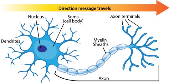
The perceptron is a simplified model of a biological neuron. In a biological neuron, there is a cell body, dendrites, and an axon. Connections between neurons, known as synapses, allow for communication. When a neuron receives enough stimuli through its dendrites, it becomes excited and sends a signal through its axon. This signal then travels to other neurons connected via synapses. Synaptic signals can be excitatory or inhibitory.
-
Inputs and Weights: Each input is associated with a weight that determines its contribution to the perceptron’s output. These weights are parameters that the perceptron adjusts during the learning process.
-
Activation function: The weighted sum of inputs is processed by an activation function, which introduces non-linearity into the network. This non-linearity is essential for neural networks to capture complex relationships between inputs and outputs, enabling them to learn complex patterns.
-
Learning Algorithm: The perceptron learns by updating its weights according to the error between the predicted label and the ground-truth label. Rosenblatt's perceptron introduced the perceptron learning rule to guide this learning process.

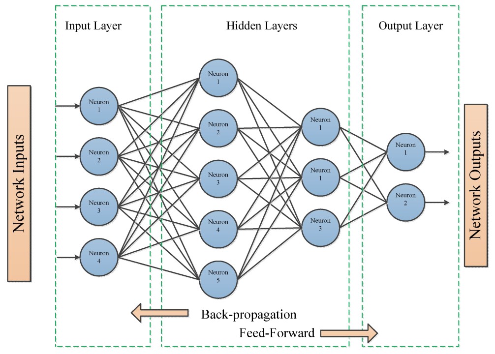
Multilayer Perceptrons (MLPs), also known as feedforward neural networks, are the simplest form of deep learning models. Their primary goal is to approximate a function
Feedforward neural networks can be thought of as a combination of multiple different functions, each of these functions represent what are know as a layer. This lets us describe a neural network in the following form:
Where
Weight initialization is a crucial aspect of training neural networks, significantly impacting the learning process. Proper initialization of weights helps mitigate common issues like vanishing and exploding gradients, which can hinder the training of deep networks.
Vanishing Gradients: In deep networks, gradients are used to update the weights during backpropagation. When gradients become too small as they are propagated backward through the layers, it results in minimal weight updates. This problem, known as vanishing gradients, causes the network to learn very slowly or even prevent learning from progressing entirely. This typically occurs in networks with activation functions that squash their input into a small range, such as the sigmoid or hyperbolic tangent (tanh) functions. These functions are prone to the saturation problem, where gradients become nearly zero for large or small input values.
Exploding Gradients: Conversely, exploding gradients occur when gradients become excessively large during backpropagation. This can lead to unstable updates and cause the network weights to diverge, making training ineffective. Exploding gradients are often observed in deep networks or in networks with large initial weights.
To address these issues, weight initialization strategies are designed to ensure that gradients neither vanish nor explode. Some common approaches include:
-
Xavier (Glorot) Initialization: This method initializes weights by drawing from a distribution with zero mean and variance inversely proportional to the number of input and output units. It is particularly effective for activation functions like sigmoid and tanh, as it helps maintain the variance of activations and gradients across layers.
-
He Initialization: Specifically designed for ReLU (Rectified Linear Unit) activation functions, He initialization draws weights from a distribution with variance proportional to the number of input units. This approach helps mitigate the issue of vanishing gradients in networks using ReLU activations.