🥇5th place solution for RSNA 2024 Lumbar Spine Degenerative Classification
Our team's approach consists of the following main components.
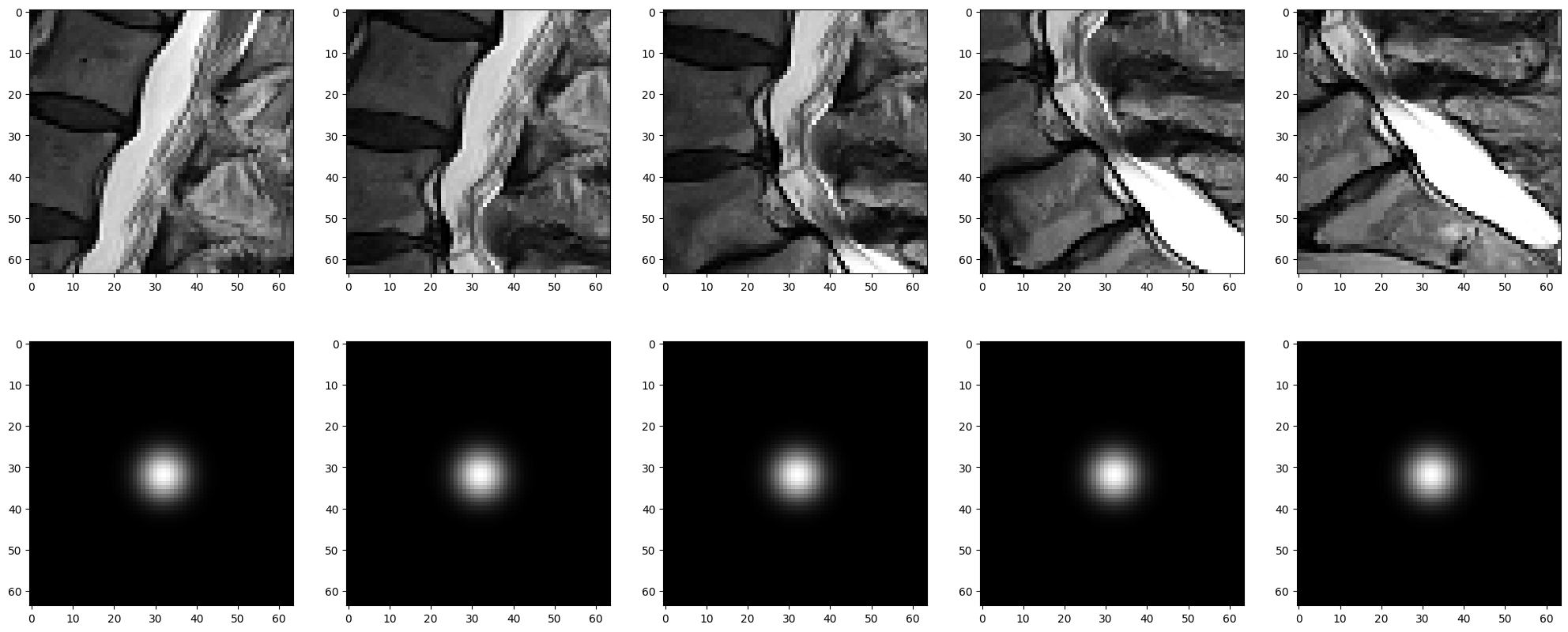
- stage1 : heatmap-based detection + gaussian-expanding-label + external-dataset
- stage2 : 2.5d model(cnn + rnn) + level-wise sequence modeling + two-step training
- augmentation : cutmix(p=1.0)
- ensemble : various backbone ensemble + tta-like ensemble
Drawing inspiration from keypoint detection, we developed a heatmap-based model to identify 25 classes. We needed to develop 3 models, each designed to predict the given labels for their respective inputs.
- sagittal_t2 -> spinal canal stenosis(5 classes)
- sagittal_t1 -> neural foraminal narrowing(10 classes)
- axial_t2 -> subarticular stenosis(10 classes)
In the early stages of the competition, we used the given points as labels, but this resulted in slower training due to class imbalance. To address this, we applied a gaussian filter to the x and y coordinates, and for the z-axis, we multiplied by 0.5 as we moved further from the target frame, effectively increasing the area of the overall labels. This helped improve the convergence speed of the models and the z-axis accuracy.
While the performance with 3d unet was good, the 2d unet combined with a sequential model demonstrated higher accuracy related to the z-axis. Therefore, we ultimately opted for a 2d unet along with a sequential model (transformer, lstm).
For the backbone, efficientnet_b5 provided the best performance. For the axial_t2, we found that increasing the maximum length to accommodate longer sequences improved performance. Additionally, leveraging the public dataset allowed us to make further improvements.
We used the detection coordinates obtained from stage 1, cropping along the z-axis by ±2 and the x, y axes by ±32, and then resized the result (5, 64, 64) -> (5, 128, 128) for use in stage 2. The structure of our model is similar to a typical 2.5d model(cnn + rnn), but our team added an additional module to model the relationships between classes. In the early stages of the competition, we modeled the 25 classes using lstm.
However, upon examining the provided data labels, we were able to make the following analysis:
When symptom 1 is present at the level, there is a high probability that symptoms 2 and 3 will also be present at the same level.
Therefore, we modified our approach to model only the classes at the same level, rather than all 25 classes. This adjustment significantly improved our score.
x = x.reshape(-1, 5, 5, self.hidden_size)
x = x.permute(0, 2, 1, 3)
x = x.reshape(-1, 5, self.hidden_size)

x, _ = self.rnn2(x)

x = x.reshape(-1, 5, 5, self.hidden_size)
x = x.permute(0, 2, 1, 3)
x = x.reshape(-1, 25, self.hidden_size)
In the later stages of the competition, we also tried concatenating the results of sequence modeling only at the same level and modeling only the same region. However, this approach did not perform better than the results from modeling only at the same level. Additionally, we implemented changes like skip connections, which we then used for our ensemble.
In the case of cnn, we experimented with models like regnet and efficientnet, but convnext demonstrated the best performance.
In the early stages of the competition, we trained our model using a loss function that closely followed the competition metric. However, this led to overfitting on the weighted labels, resulting in poor auc score. To improve the auc while still performing well on the competition metric, our team implemented a two-step training approach.
1st-step(pretraining) We focused on maximizing the auc score by training the model's overall parameters without using weighted loss and any loss.
2nd-step(finetuning) We employed weighted loss and any loss, freezing the model's backbone and training only the head parameters to optimize for the competition metric.
Through this method, our team was able to significantly improve our scores compared to simply training with weighted loss and any loss.
When training stage 2, we observed that the model quickly began to overfit. To prevent overfitting, we tried various methods, including flip, rotate, brightness, contrast, blur, and mixup. Among these, cutmix played the most significant role in increasing the auc score. In fact, using cutmix with p=1.0 resulted in the highest auc score.
Additionally, we experimented with various methods, such as randomly adding ±1 at the z from stage1 or flipping the left and right labels. However, these approaches did not result in significant score improvements.
Based on these methods, we developed various stage 1 and stage 2 models and performed an ensemble.
- stage1 : max length
- stage1 : cnn backbone(regnety_002, efficientnet_b5)
- stage1 : whether it has fixed (x, y) coordinates or dynamic (x, y) coordinates according to the z-axis.
- stage2 : rnn modeling(skip connection, sequence modeling axis)
- stage2 : cnn backbone(convnext_small, convnext_tiny, caformer_s18, pvt_v2_b3)
Additionally, the ensemble method that yielded the highest score on the private leaderboard was similar to test-time augmentation (tta). Instead of combining the stage 1 models developed by team members and passing them to stage 2 models, we inferred stage 2 models for each individual stage 1 model and then performed an ensemble.
- adding the mask from stage 1 as the stage 2's cnn channel
- bigger cnn backbone for stage2
- label smoothing