bayesplot

Overview

bayesplot is an R package providing an extensive library of plotting functions for use after fitting Bayesian models (typically with MCMC). The plots created by bayesplot are ggplot objects, which means that after a plot is created it can be further customized using various functions from the ggplot2 package.

Currently bayesplot offers a variety of plots of posterior draws, visual MCMC diagnostics, graphical posterior (or prior) predictive checking, and general plots of posterior (or prior) predictive distributions.

The idea behind bayesplot is not only to provide convenient functionality for users, but also a common set of functions that can be easily used by developers working on a variety of packages for Bayesian modeling, particularly (but not necessarily) those powered by RStan.

Getting started

If you are just getting started with bayesplot we recommend starting with the tutorial vignettes, the examples throughout the package documentation, and the paper Visualization in Bayesian workflow:

• Gabry J, Simpson D, Vehtari A, Betancourt M, Gelman A (2019). Visualization in Bayesian workflow. J. R. Stat. Soc. A, 182: 389-402. doi:10.1111/rssa.12378. (journal version, arXiv preprint, code on GitHub)

Resources

• mc-stan.org/bayesplot (online documentation, vignettes)
• Ask a question (Stan Forums on Discourse)
• Open an issue (GitHub issues for bug reports, feature requests)

Contributing

We are always looking for new contributors! See CONTRIBUTING.md for details and/or reach out via the issue tracker.

Installation

• Install from CRAN:

install.packages("bayesplot")

• Install latest development version from GitHub (requires devtools package):

if (!require("devtools")) {
  install.packages("devtools")
}
devtools::install_github("stan-dev/bayesplot", dependencies = TRUE, build_vignettes = FALSE)

This installation won't include the vignettes (they take some time to build), but all of the vignettes are available online at mc-stan.org/bayesplot/articles.

Examples

Some quick examples using MCMC draws obtained from the rstanarm and rstan packages.

library("bayesplot")
library("rstanarm")
library("ggplot2")

fit <- stan_glm(mpg ~ ., data = mtcars)
posterior <- as.matrix(fit)

plot_title <- ggtitle("Posterior distributions",
                      "with medians and 80% intervals")
mcmc_areas(posterior, 
           pars = c("cyl", "drat", "am", "wt"), 
           prob = 0.8) + plot_title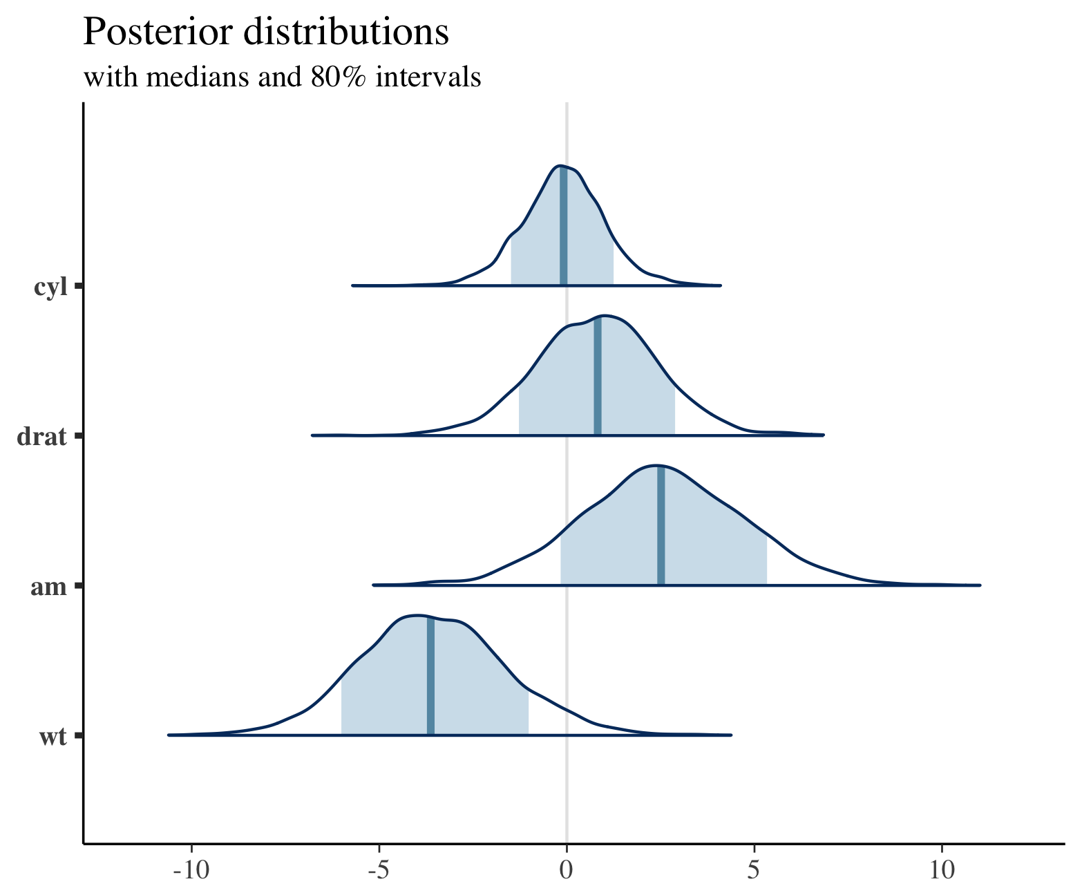

color_scheme_set("red")
ppc_dens_overlay(y = fit$y, 
                 yrep = posterior_predict(fit, draws = 50))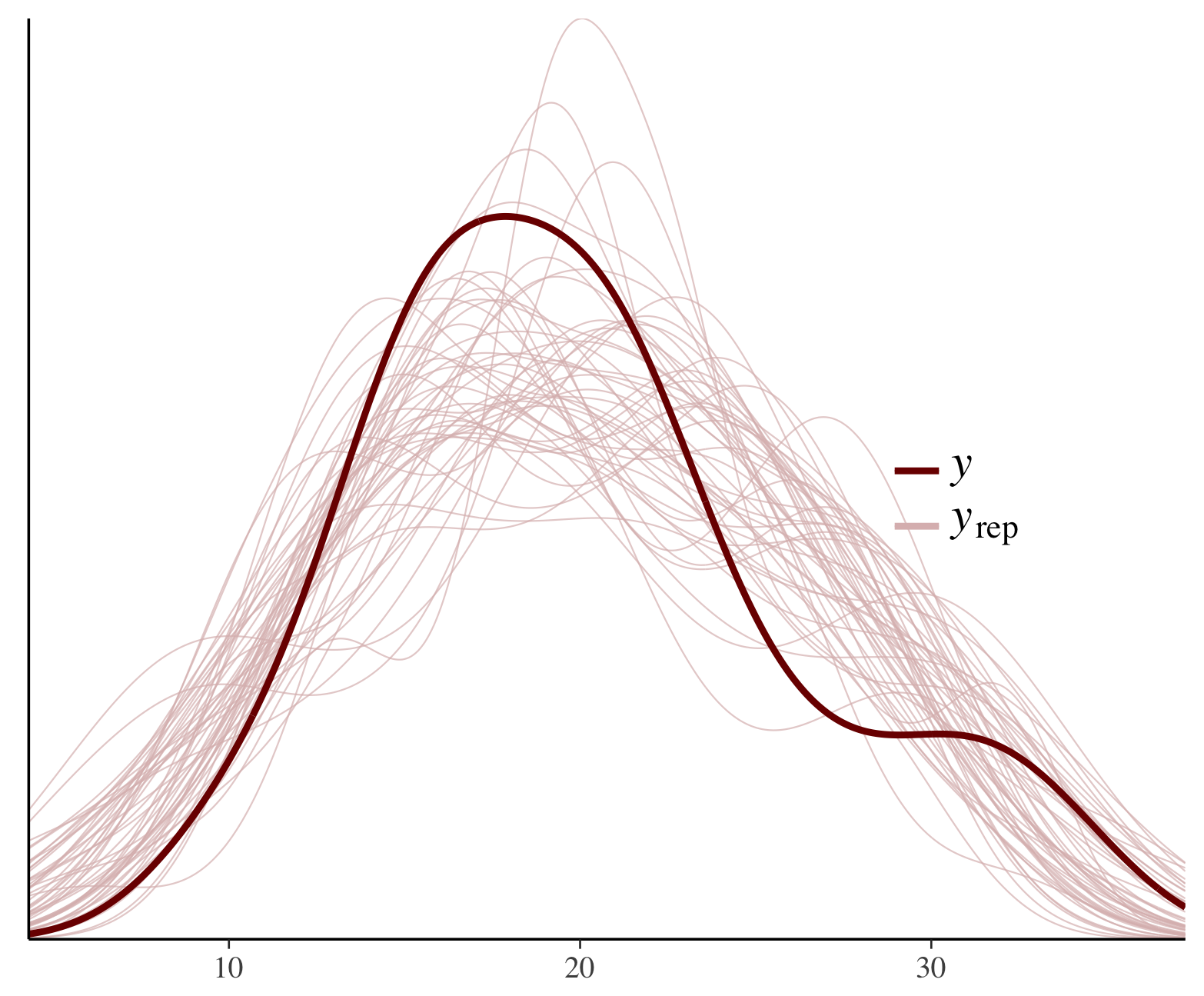

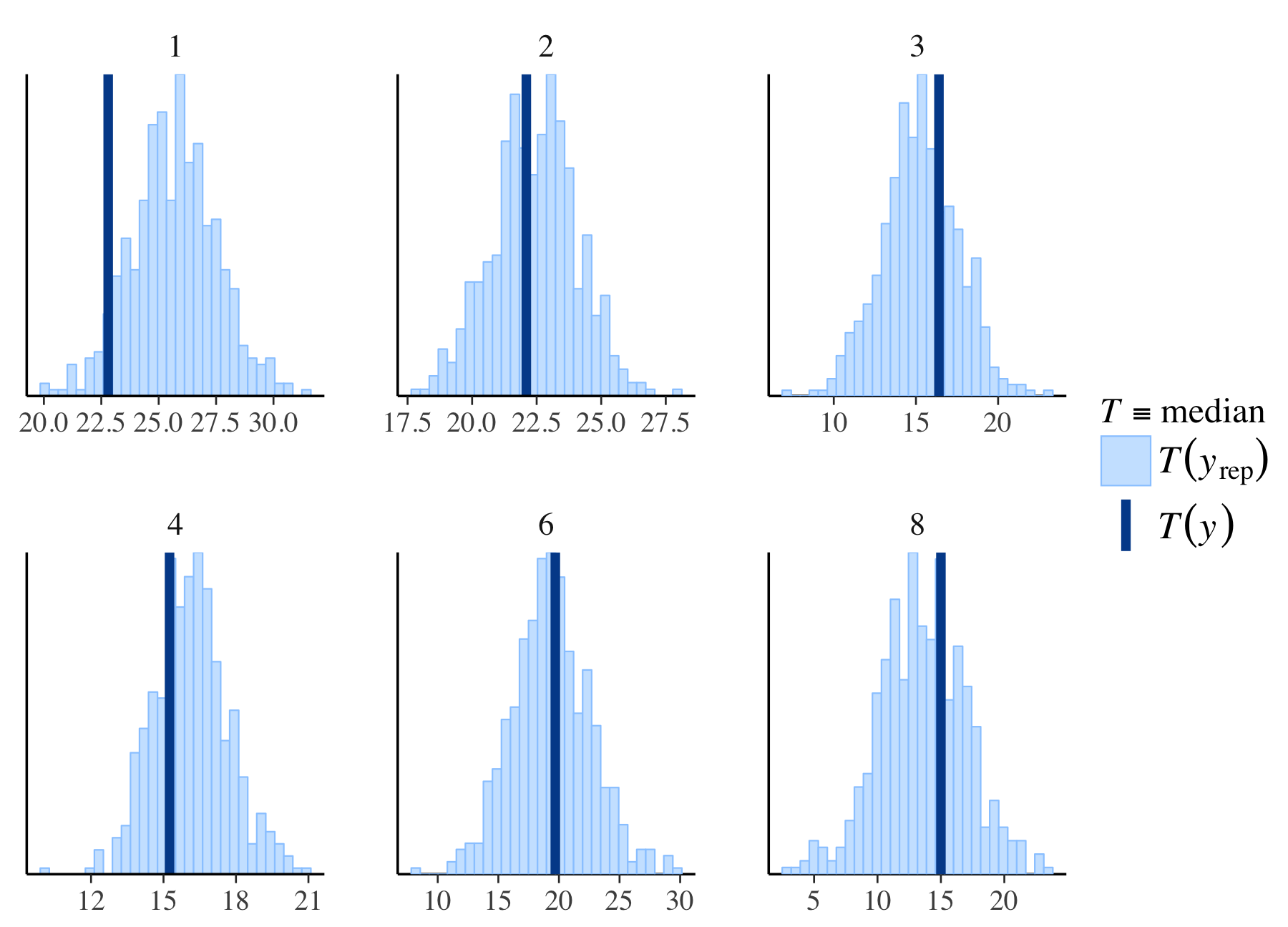
# also works nicely with piping
library("dplyr")
color_scheme_set("brightblue")
fit %>% 
  posterior_predict(draws = 500) %>%
  ppc_stat_grouped(y = mtcars$mpg, 
                   group = mtcars$carb, 
                   stat = "median")

# with rstan demo model
library("rstan")
fit2 <- stan_demo("eight_schools", warmup = 300, iter = 700)
posterior2 <- extract(fit2, inc_warmup = TRUE, permuted = FALSE)

color_scheme_set("mix-blue-pink")
p <- mcmc_trace(posterior2,  pars = c("mu", "tau"), n_warmup = 300,
                facet_args = list(nrow = 2, labeller = label_parsed))
p + facet_text(size = 15)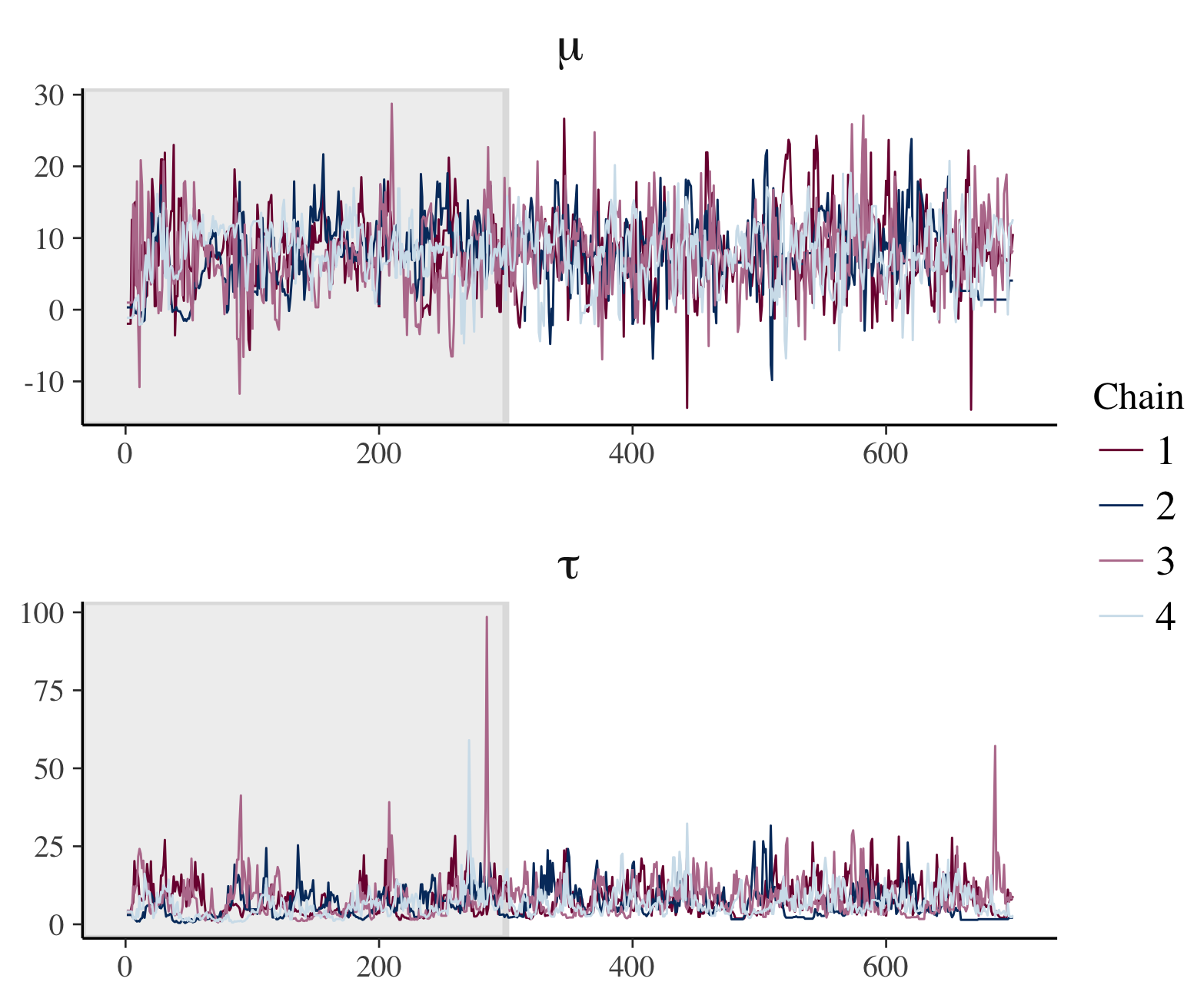

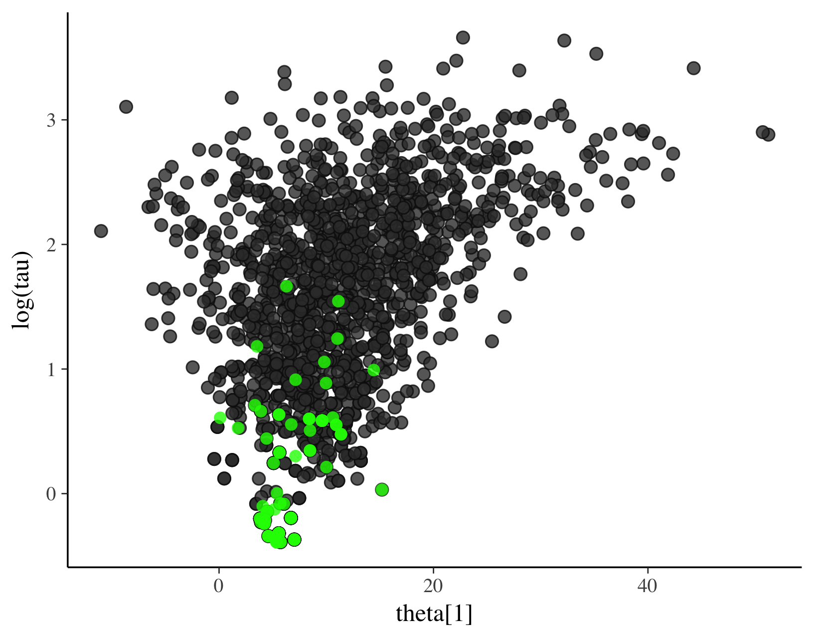
# scatter plot also showing divergences
color_scheme_set("darkgray")
mcmc_scatter(
  as.matrix(fit2),
  pars = c("tau", "theta[1]"), 
  np = nuts_params(fit2), 
  np_style = scatter_style_np(div_color = "green", div_alpha = 0.8)
)

color_scheme_set("red")
np <- nuts_params(fit2)
mcmc_nuts_energy(np) + ggtitle("NUTS Energy Diagnostic")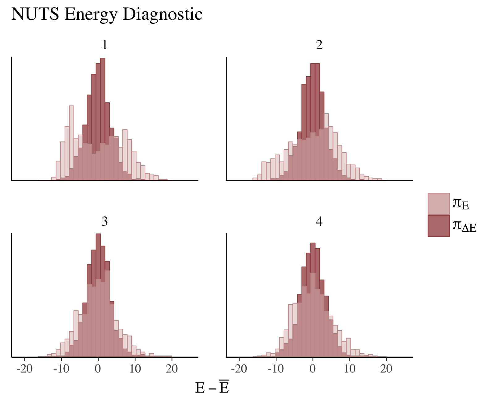

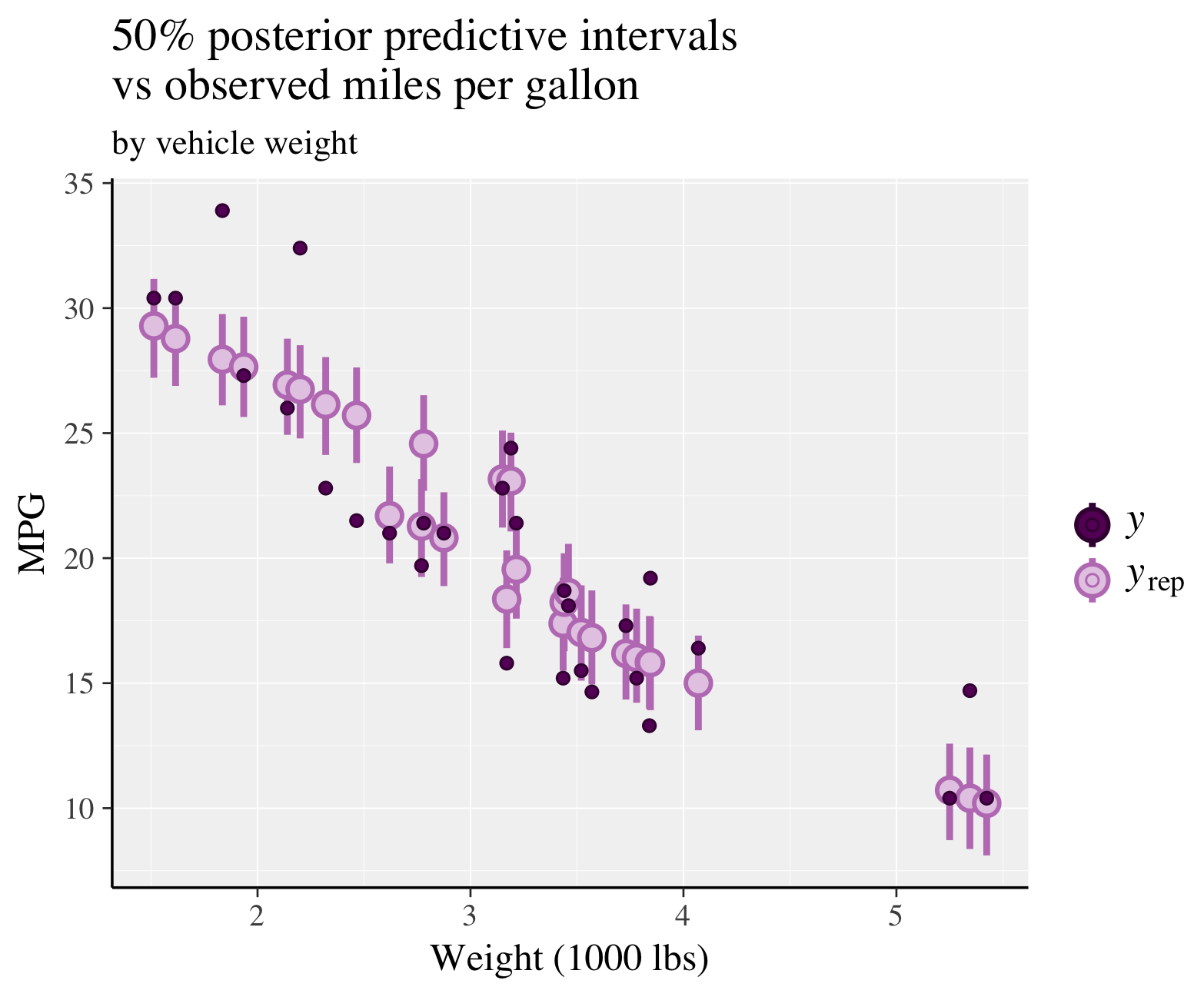
# another example with rstanarm
color_scheme_set("purple")

fit <- stan_glmer(mpg ~ wt + (1|cyl), data = mtcars)
ppc_intervals(
  y = mtcars$mpg,
  yrep = posterior_predict(fit),
  x = mtcars$wt,
  prob = 0.5
) +
  labs(
    x = "Weight (1000 lbs)",
    y = "MPG",
    title = "50% posterior predictive intervals \nvs observed miles per gallon",
    subtitle = "by vehicle weight"
  ) +
  panel_bg(fill = "gray95", color = NA) +
  grid_lines(color = "white")