Fourier Series MATLAB Tool

This project is supervised by Dr. Tak Kwong WONG and use as teaching material. This project aims to build a useful MATLAB tool for studying the Fourier series of any function and some special phenomenon.

What is Fourier Series...

The Fourier series is named in honor of Jean-Baptiste Joseph Fourier (1768–1830), and the series approximate an arbitrary function in an interval or .
Wikipedia

Different Types of Fourier Series

Fourier Sine Series on

Fourier Cosine Series on

Fourier (Sine and Cosine) Series on

Getting Started

Dependencies

• MATLAB (R2021a or latest version)
• Symbolic Math Toolbox (link)

Installing

1. Download
2. Place the folder under the MATLAB working directory. If you not sure where is the directory, you can type the following in the command window of MATLAB.

>> pwd

ans =

    '/Users/YourName/Document/Folder/MATLAB'

>>

3. Open initializer.m and run it For first time you run, you will see a message
   
   Click Change Folder and the MATLAB working directory will be redirected to Fourier_Series_tool-main folder.
   

4. Check the working directory is it correct.

>> pwd

ans =

    '/Users/YourName/Document/Folder/MATLAB/Fourier_Series_tool-main'

>>

For any question, please refert to MATLAB Help Center. Link

Executing program

1. edit the parameter in initializer.m and run it. Then it will create a folder.

/Fourier_Series_YOUR_FUNCTION_(n=123)[INTERVAL_START, INTERVAL_END]SERIES_TYPE

For example,
Fourier_Series_piecewise(x in Dom//Interval([1], [2]) | x in Dom//Interval([3], [4]) | x in Dom//Interval([5], [6]), 1, symtrue, 0)(n=1000)[0, 6.2832]_Sine

3. run Fourier_Series_Coefficients.m and then it will export a .csv file that contain all coefficients.
4. run Fourier_Series_Result.m
5. run Fourier_Series_Plot_and_Animation.m and then it will return a animation .gif file and the snapshot in /snapshot_of_gif folder.

Example 1 (Plot a gif of Fourier Series)

The show the Fourier sine series on interval from n = 1 to n = 50.

1. Open initializer.m and change the parameter as following, inculding f(x), interval_start, interval_end, n, series_type, and function_name.

%%%%%%%%%%%%%%%%%%%%%%%%%%%%%%%%%%%%%%%%%%%%%%%%%%%%%%%%%%%%%%%%%%%%%

% Define f(x)
syms x
f = sin(2*x) + x^2;

% Interval and number of series
interval_start = 0;
interval_end = 2*pi;
n = 50;

% Series type choose from ['Sine','Cosine','Sine_and_Cosine']
series_type = 'Sine';

% Function name
function_name = 'function 1';

%%%%%%%%%%%%%%%%%%%%%%%%%%%%%%%%%%%%%%%%%%%%%%%%%%%%%%%%%%%%%%%%%%%%%

For the detail of creating symbolic functions on MATLAB, please refer to https://www.mathworks.com/help/symbolic/syms.html#buoeaym-1

2. Run initializer.m and there will be a folder Fourier_Series_function 1_(n=50)_[0, 6.2832]_Sine and a info.txt file. The variables will be stored in MATLAB.

>> initializer
Initialization finished.

3. Run Fourier_Series_Coefficients.m and it will take some time to compute each of the coefficients of Fourier series, i.e. or

>> Fourier_Series_Coefficients
The Fourier Series Coefficients have been calculated.
Exported! csv file name: Fourier_Coefficients_function 1_(n=50)_[0, 6.2832]_Sine.csv
Exported! png file name: Fourier_Coefficients_function 1_(n=50)_[0, 6.2832]_Sine.png
Elapsed time is 4.637936 seconds.

It will export .csv and .png files of the coefficients. 4. Run Fourier_Series_Result.m. It will based on the pervious coefficients.

>> Fourier_Series_Result
Fourier Series result from 0 to 50 have been generated.

In MATLAB, there is the random partition on the interval for plotting the graph, i.e., .
The variable result_ind_terms contain the value of different terms.

The result_ind_terms matrix


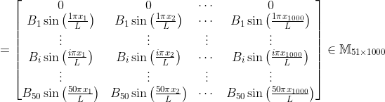
The result_sum_terms matrix

The row refer to the Fourier series value on each partition point .

5. Run Fourier_Series_Plot_and_Animation.m. It plot all series and create the gif. This takes some time.

>> Fourier_Series_Plot_and_Animation
Animation done!

To view the plotting process, you can change h = figure('visible', 'off') to be h = figure('visible', 'on').

6. After then, there will be Fourier_Series_function 1_(n=50)_[0, 6.2832]_Sine.gif in the folder and /snapshot_og_gif/ folder contain all snapshot of gif.

Example 2 (Import existing Fourier series coefficients from external sources)

Given you would import a Fourier Coefficients .csv file for some function . For example, a coefficient of Fourier Sine series,

n	B_n
0	0
1	4
2	2
3	1.33333333333
4	1
5	0.8
...	...

1. First, you need to initialize the parameter in initializer.m and then run it. There will be a folder created.
2. To import the .csv file, you need to place the file under the folder.
3. Edit the parameter in Import_the_Fourier_Coefficients_csv.m

%%%%%%%%%%%%%%%%%%%%%%%%%%%%%%%%%%%%%%%%%%%%%%%%%%%%%%%%%%%%%%%%%%%%%
% Make sure the file name and the folder path is correct
folder_name_import = 'Fourier_Series_Triangle_and_Semicircle_(n=400)_[0, 6.2832]_Sine';
file_name_import = 'Fourier_Coefficients_Triangle_and_Semicircle_(n=400)_[0, 6.2832]_Sine.csv';
%%%%%%%%%%%%%%%%%%%%%%%%%%%%%%%%%%%%%%%%%%%%%%%%%%%%%%%%%%%%%%%%%%%%%

4. Run it

>> Import_the_Fourier_Coefficients_csv
Imported!
Exported! png file name: Fourier_Coefficients_Triangle_and_Semicircle_(n=400)_[0, 6.2832]_Sine.png
>> 

5. Run Fourier_Series_Result.m and Fourier_Series_Plot_and_Animation.m as usual.

Example 3 (Plot different n terms in one plot)

1. Run initializer.m,Fourier_Series_Coefficients.m,Fourier_Series_Result.m,and Fourier_Series_Plot_and_Animation.m as usual.
2. open Different_Fourier_Series_plot and edit the following parameter

%%%%%%%%%%%%%%%%%%%%%%%%%%%%%%%%%%%%%%%%%%%%%%%%%%%%%%%%%%%%%%%%%%%%%
% list of n to plot
list_of_n_to_plot = [1,2,4,10,50,200];
%%%%%%%%%%%%%%%%%%%%%%%%%%%%%%%%%%%%%%%%%%%%%%%%%%%%%%%%%%%%%%%%%%%%%

Change axis_boundary in case you need.

3. Run it and then different .png plot will be in the folder.

Example 4 (Zoom in to show Gibbs Phenomenon)

Gibbs_Phenomenon_zoom_in_Animation.m is a independent programme to show Gibbs phenomenon (Wikipedia) in . It will show the near 9 percent of the jump at the a jump discontinuity.

Example:

Example 5 (Animaation of wave equation solution)

The homogeneous Dirichlet conditions for the wave equation with some initial conditions:

By method of separation of variables, the solutio will be

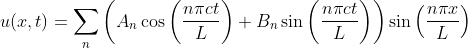
where the coefficients is the Fourier coefficients of Fourier sine series of , that is , and the coefficients is .

1. open Homogeneous_Dirichlet_Conditions_for_Wave_Equation_with_IC and edit the following parameter

%%%%%%%%%%%%%%%%%%%%%%%%%%%%%%%%%%%%%%%%%%%%%%%%%%%%%%%%%%%%%%%%%%%%%%%
% Define the parameter
syms x;
c = 10;
L = 2*pi;
phi = 0.5*x^2;
psi = x;
n = 500;
t_end = 10;

function_name = 'testing_result_v7';

% axis tight manual
axis_boundary = [0,L,-10,30];

%%%%%%%%%%%%%%%%%%%%%%%%%%%%%%%%%%%%%%%%%%%%%%%%%%%%%%%%%%%%%%%%%%%%%%%

2. run it and then the result will be saved under the folder.

Reference: W.A. Strauss: Partial Differential Equations: An Introduction, Hoboken, N.J. : Wiley c2008 2nd ed. Chapter 4

Authors

@twn-wi11i4m

Version History

• Ver 1.0
  • Initial Release
• Ver 2.0
  • Improve the algorithm to compute the Fourier coefficients.
  • Adding the wave equation simulator

License

This project is licensed under the MIT License - see the LICENSE.md file for details

Acknowledgments

Special thanks to Dr. Wong, who give the idea and comment on this project.