X‐Drive Controller

Robot Dynamics Model

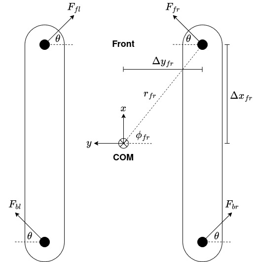
We define the force from a given thruster $T$ as $F_T$ and its $x$ and $y$ components as $F_{Tx}$ and $F_{Ty}$. The xy location of the corresponding thruster is defined as $\Delta x_T$ and $\Delta y_T$, its angle from the center of mass as $\phi_T=\frac{\Delta x_T}{\Delta y_T}$, and its distance from the boat's center of mass as $r_T=\sqrt{\Delta x_T^2+\Delta y_T^2}$. Finally, the angle of the thrusters are given by $\theta$, and the drag force is calculated as

$$F_d=\frac{1}{2}\rho v^2c_dA=cv^2$$

where $\rho$ is the fluid density, $v$ is the relative velocity of the fluid, $c_d$ is the drag coefficient, and $A$ is the reference area [1]. We empirically determine the product of these constants $c$. Using these variables, the net forces and torque are calculated by

$$\sum F_x=F_{frx}+F_{blx}+F_{flx}+F_{brx}-F_{dx}=(F_{frx}+F_{blx}+F_{flx}+F_{brx})\sin\theta-F_{dx}$$ $$\sum F_y=F_{fry}+F_{bly}-F_{fly}-F_{bry}-F_{dy}=(F_{fry}+F_{bly}-F_{fly}-F_{bry})\cos\theta-F_{dy}$$ $$\sum \tau=F_{fr}r_{fr}\sin(\theta+\phi_{fr})-F_{bl}r_{bl}\sin(\theta+\phi_{bl})-F_{fl}r_{fl}\sin(\theta+\phi_{fl})+F_{br}r_{br}\sin(\theta+\phi_{br})-\tau_d$$

For a given target velocity, the forces are at equilibrium, so

$$\sum F_x=0\implies (F_{frx}+F_{blx}+F_{flx}+F_{brx})\sin\theta=F_{dx}$$ $$\sum F_y=0\implies (F_{fry}+F_{bly}-F_{fly}-F_{bry})\cos\theta=F_{dy}$$ $$\sum \tau=0\implies F_{fr}r_{fr}\sin(\theta+\phi_{fr})-F_{bl}r_{bl}\sin(\theta+\phi_{bl})-F_{fl}r_{fl}\sin(\theta+\phi_{fl})+F_{br}r_{br}\sin(\theta+\phi_{br})=\tau_d$$

The force from each thruster is approximately proportional to the control input, so $F_T=b_Tu_T$ where $b_T$ is the maximum force for each thruster (approximately 40N for the Blue Robotics T200 thrusters) and $u_T\in[-1,1]$ is the control input [1]. Thus, we can rewrite these equations as a single matrix equation:

$$Bu=Cv^2$$

where

$$B=\begin{bmatrix} b_{fr}\sin\theta & b_{bl}\sin\theta & b_{fl}\sin\theta & b_{br}\sin\theta \\ b_{fr}\cos\theta & b_{bl}\cos\theta & -b_{fl}\cos\theta & -b_{br}\cos\theta \\ b_{fr}r_{fr}\sin(\theta+\phi_{fr}) & -b_{bl}r_{bl}\sin(\theta+\phi_{bl}) & -b_{fl}r_{fl}\sin(\theta+\phi_{fl}) & b_{br}r_{br}\sin(\theta+\phi_{br}) \end{bmatrix}$$

$$u=\begin{bmatrix}u_{fr} & u_{bl} & u_{fl} & u_{br}\end{bmatrix}^T$$

$$v=\begin{bmatrix}v_x & v_y & \omega_z\end{bmatrix}^T$$

$$C=\begin{bmatrix} C_x & 0 & 0 \\ 0 & C_y & 0 \\ 0 & 0 & C_z \end{bmatrix}$$

and $C_x,C_y,C_z$ are empirically determined constants. Given a target velocity $v$, solving for $u$ returns the desired control inputs.

Controller Optimization

Since the equation above is underdetermined (more variables than equations), there are multiple solutions to the problem. Thus, we formulate this equation into an optimization problem to find the solution with minimum norm using the python scipy library:

$$u^\star=\underset{u \in \mathbb{R}^4}{\mathrm{argmin}}\lVert u\rVert$$ $$\text{s.t. } u\in[-1,1],\quad Bu=Cv^2$$

References

[1] D. A. Klahn, “Design and Implementation of Control and Perception Subsystems for an Autonomous Surface Vehicle for Aquaculture,” Mit.edu, Jun. 2023, doi: https://hdl.handle.net/1721.1/151394.